Your favourite package for getting model outputs directly into publication ready tables is now available on CRAN. They make you work for it! Thank you to all that helped. The development version will continue to be available from github.
Elegant regression results tables and plots in R: the finalfit package
The finafit package brings together the day-to-day functions we use to generate final results tables and plots when modelling. I spent many years repeatedly manually copying results from R analyses and built these functions to automate our standard healthcare data workflow. It is particularly useful when undertaking a large study involving multiple different regression analyses. When combined with RMarkdown, the reporting becomes entirely automated. Its design follows Hadley Wickham’s tidy tool manifesto.
Installation and Documentation
The full documentation is now here: finalfit.org
The code lives on GitHub.
You can install finalfit from CRAN with:
install.packages("finalfit")
It is recommended that this package is used together with dplyr, which is a dependent.
Some of the functions require rstan and boot. These have been left as Suggests rather than Depends to avoid unnecessary installation. If needed, they can be installed in the normal way:
install.packages("rstan")
install.packages("boot")
To install off-line (or in a Safe Haven), download the zip file and use devtools::install_local().
Main Features
1. Summarise variables/factors by a categorical variable
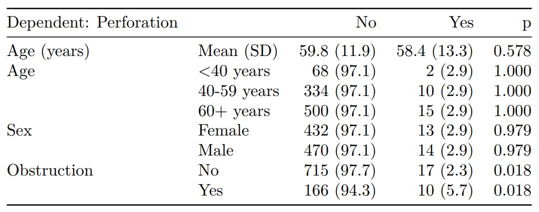
summary_factorlist() is a wrapper used to aggregate any number of explanatory variables by a single variable of interest. This is often “Table 1” of a published study. When categorical, the variable of interest can have a maximum of five levels. It uses Hmisc::summary.formula().
library(finalfit)
library(dplyr)

# Load example dataset, modified version of survival::colon
data(colon_s)

# Table 1 - Patient demographics by variable of interest ----
explanatory = c("age", "age.factor",
  "sex.factor", "obstruct.factor")
dependent = "perfor.factor" # Bowel perforation
colon_s %>%
  summary_factorlist(dependent, explanatory,
  p=TRUE, add_dependent_label=TRUE)
See other options relating to inclusion of missing data, mean vs. median for continuous variables, column vs. row proportions, include a total column etc.
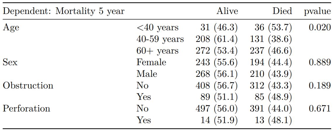
summary_factorlist() is also commonly used to summarise any number of variables by an outcome variable (say dead yes/no).
# Table 2 - 5 yr mortality ----
explanatory = c("age.factor",
  "sex.factor",
  "obstruct.factor")
dependent = 'mort_5yr'
colon_s %>%
  summary_factorlist(dependent, explanatory,
  p=TRUE, add_dependent_label=TRUE)
Tables can be knitted to PDF, Word or html documents. We do this in RStudio from a .Rmd document. Example chunk:
```{r, echo = FALSE, results='asis'}
knitr::kable(example_table, row.names=FALSE,
    align=c("l", "l", "r", "r", "r", "r"))
```
2. Summarise regression model results in final table format
The second main feature is the ability to create final tables for linear (lm()), logistic (glm()), hierarchical logistic (lme4::glmer()) and
Cox proportional hazards (survival::coxph()) regression models.
The finalfit() “all-in-one” function takes a single dependent variable with a vector of explanatory variable names (continuous or categorical variables) to produce a final table for publication including summary statistics, univariable and multivariable regression analyses. The first columns are those produced by summary_factorist(). The appropriate regression model is chosen on the basis of the dependent variable type and other arguments passed.
Logistic regression: glm()
Of the form: glm(depdendent ~ explanatory, family="binomial")
explanatory = c("age.factor", "sex.factor",
  "obstruct.factor", "perfor.factor")
dependent = 'mort_5yr'
colon_s %>%
  finalfit(dependent, explanatory)
Logistic regression with reduced model: glm()
Where a multivariable model contains a subset of the variables included specified in the full univariable set, this can be specified.
explanatory = c("age.factor", "sex.factor",
  "obstruct.factor", "perfor.factor")
explanatory_multi = c("age.factor",
  "obstruct.factor")
dependent = 'mort_5yr'
colon_s %>%
  finalfit(dependent, explanatory,
  explanatory_multi)
Mixed effects logistic regression: lme4::glmer()
Of the form: lme4::glmer(dependent ~ explanatory + (1 | random_effect), family="binomial")
Hierarchical/mixed effects/multilevel logistic regression models can be specified using the argument random_effect. At the moment it is just set up for random intercepts (i.e. (1 | random_effect), but in the future I’ll adjust this to accommodate random gradients if needed (i.e. (variable1 | variable2).
explanatory = c("age.factor", "sex.factor",
  "obstruct.factor", "perfor.factor")
explanatory_multi = c("age.factor", "obstruct.factor")
random_effect = "hospital"
dependent = 'mort_5yr'
colon_s %>%
  finalfit(dependent, explanatory,
  explanatory_multi, random_effect)
Cox proportional hazards: survival::coxph()
Of the form: survival::coxph(dependent ~ explanatory)
explanatory = c("age.factor", "sex.factor",
"obstruct.factor", "perfor.factor")
dependent = "Surv(time, status)"
colon_s %>%
  finalfit(dependent, explanatory)
Add common model metrics to output
metrics=TRUE provides common model metrics. The output is a list of two dataframes. Note chunk specification for output below.
explanatory = c("age.factor", "sex.factor",
  "obstruct.factor", "perfor.factor")
dependent = 'mort_5yr'
colon_s %>%
  finalfit(dependent, explanatory,
  metrics=TRUE)
```{r, echo=FALSE, results="asis"}
knitr::kable(table7[[1]], row.names=FALSE, align=c("l", "l", "r", "r", "r"))
knitr::kable(table7[[2]], row.names=FALSE)
```
Rather than going all-in-one, any number of subset models can be manually added on to a summary_factorlist() table using finalfit_merge(). This is particularly useful when models take a long-time to run or are complicated.
Note the requirement for fit_id=TRUE in summary_factorlist(). fit2df extracts, condenses, and add metrics to supported models.
explanatory = c("age.factor", "sex.factor",
  "obstruct.factor", "perfor.factor")
explanatory_multi = c("age.factor", "obstruct.factor")
random_effect = "hospital"
dependent = 'mort_5yr'

# Separate tables
colon_s %>%
  summary_factorlist(dependent,
  explanatory, fit_id=TRUE) -> example.summary

colon_s %>%
  glmuni(dependent, explanatory) %>%
  fit2df(estimate_suffix=" (univariable)") -> example.univariable

colon_s %>%
  glmmulti(dependent, explanatory) %>%
  fit2df(estimate_suffix=" (multivariable)") -> example.multivariable

colon_s %>%
  glmmixed(dependent, explanatory, random_effect) %>%
  fit2df(estimate_suffix=" (multilevel)") -> example.multilevel

# Pipe together
example.summary %>%
  finalfit_merge(example.univariable) %>%
  finalfit_merge(example.multivariable) %>%
  finalfit_merge(example.multilevel) %>%
  select(-c(fit_id, index)) %>% # remove unnecessary columns
  dependent_label(colon_s, dependent, prefix="") # place dependent variable label
Bayesian logistic regression: with `stan`
Our own particular rstan models are supported and will be documented in the future. Broadly, if you are running (hierarchical) logistic regression models in Stan with coefficients specified as a vector labelled beta, then fit2df() will work directly on the stanfit object in a similar manner to if it was a glm or glmerMod object.
3. Summarise regression model results in plot
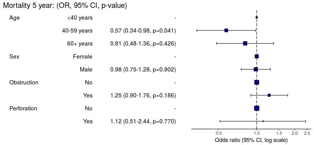
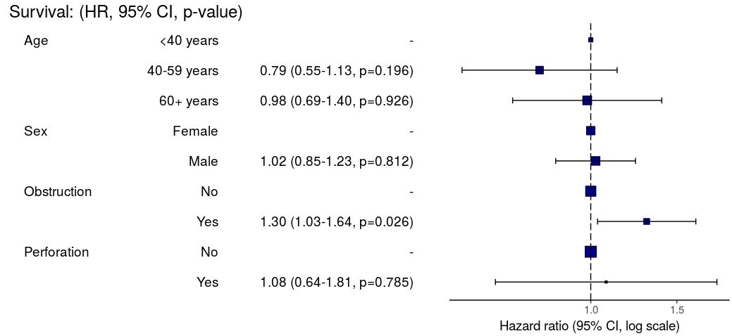
Models can be summarized with odds ratio/hazard ratio plots using or_plot, hr_plot and surv_plot.
OR plot
# OR plot
explanatory = c("age.factor", "sex.factor",
  "obstruct.factor", "perfor.factor")
dependent = 'mort_5yr'
colon_s %>%
  or_plot(dependent, explanatory)
# Previously fitted models (`glmmulti()` or
# `glmmixed()`) can be provided directly to `glmfit`
HR plot
# HR plot
explanatory = c("age.factor", "sex.factor",
  "obstruct.factor", "perfor.factor")
dependent = "Surv(time, status)"
colon_s %>%
  hr_plot(dependent, explanatory, dependent_label = "Survival")
# Previously fitted models (`coxphmulti`) can be provided directly using `coxfit`
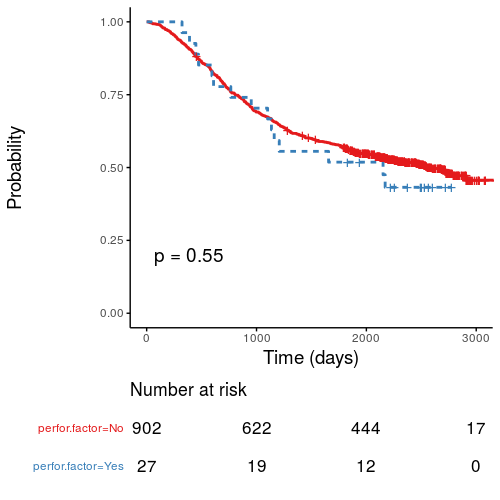
Kaplan-Meier survival plots
KM plots can be produced using the library(survminer)
# KM plot
explanatory = c("perfor.factor")
dependent = "Surv(time, status)"
colon_s %>%
  surv_plot(dependent, explanatory,
  xlab="Time (days)", pval=TRUE, legend="none")
Notes
Use Hmisc::label() to assign labels to variables for tables and plots.
label(colon_s$age.factor) = "Age (years)"
Export dataframe tables directly or to R Markdown knitr::kable().
Note wrapper summary_missing() is also useful. Wraps mice::md.pattern.
colon_s %>%
  summary_missing(dependent, explanatory)
Development will be on-going, but any input appreciated.
P-values from random effects linear regression models
lme4::lmer is a useful frequentist approach to hierarchical/multilevel linear regression modelling. For good reason, the model output only includes t-values and doesn’t include p-values (partly due to the difficulty in estimating the degrees of freedom, as discussed here).
Yes, p-values are evil and we should continue to try and expunge them from our analyses. But I keep getting asked about this. So here is a simple bootstrap method to generate two-sided parametric p-values on the fixed effects coefficients. Interpret with caution.
library(lme4)

# Run model with lme4 example data
fit = lmer(angle ~ recipe + temp + (1|recipe:replicate), cake)

# Model summary
summary(fit)

# lme4 profile method confidence intervals
confint(fit)

# Bootstrapped parametric p-values
boot.out = bootMer(fit, fixef, nsim=1000) #nsim determines p-value decimal places
p = rbind(
  (1-apply(boot.out$t<0, 2, mean))*2,
  (1-apply(boot.out$t>0, 2, mean))*2)
apply(p, 2, min)

# Alternative "pipe" syntax
library(magrittr)

lmer(angle ~ recipe + temp + (1|recipe:replicate), cake) %>%
  bootMer(fixef, nsim=100) %$%
  rbind(
  (1-apply(t<0, 2, mean))*2,
  (1-apply(t>0, 2, mean))*2) %>%
  apply(2, min)
RStudio and GitHub
Version control has become essential for me keeping track of projects, as well as collaborating. It allows backup of scripts and easy collaboration on complex projects. RStudio works really well with Git, an open source open source distributed version control system, and GitHub, a web-based Git repository hosting service. I was always forget how to set up a repository, so here’s a reminder.
This example is done on RStudio Server, but the same procedure can be used for RStudio desktop. Git or similar needs to be installed first, which is straight forward to do.
Setup Git on RStudio and Associate with GitHub
In RStudio, Tools -> Version Control, select Git.
In RStudio, Tools -> Global Options, select Git//SVN tab. Ensure the path to the Git executable is correct. This is particularly important in Windows where it may not default correctly (e.g. C:/Program Files (x86)/Git/bin/git.exe).
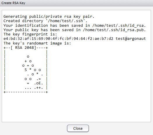
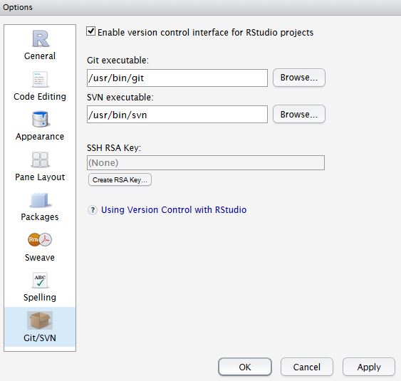 Now hit, Create RSA Key …
Click, View public key, and copy the displayed public key.
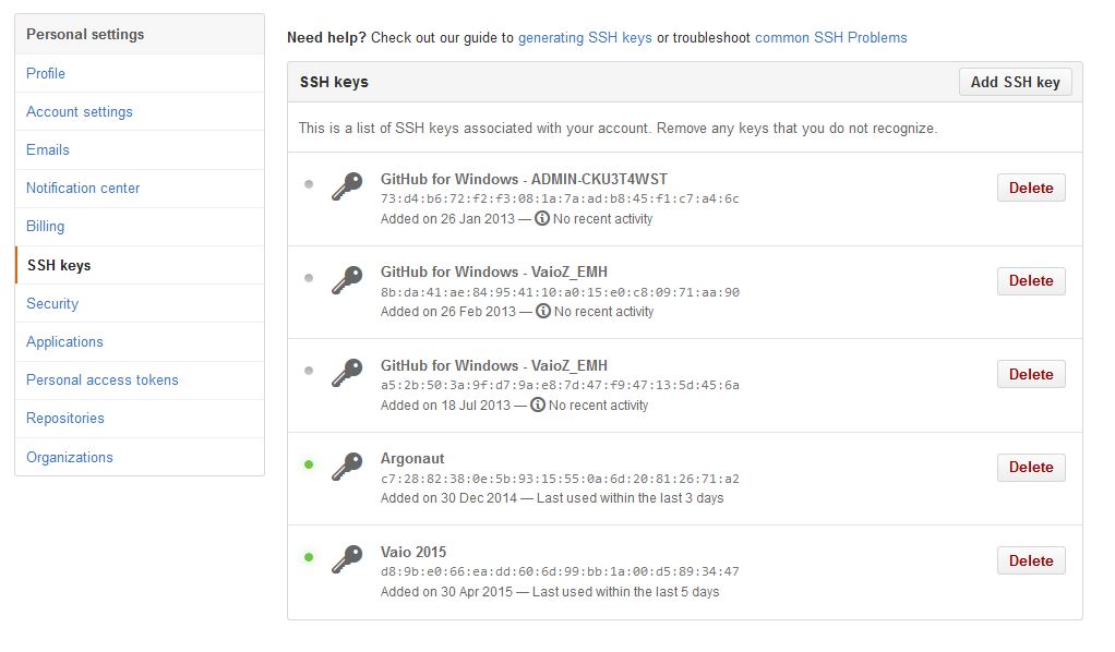
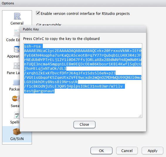 If you haven’t already, create a GitHub account. Open your account settings and click the SSH keys tab. Click Add SSH key. Paste in the public key you have copied from RStudio.
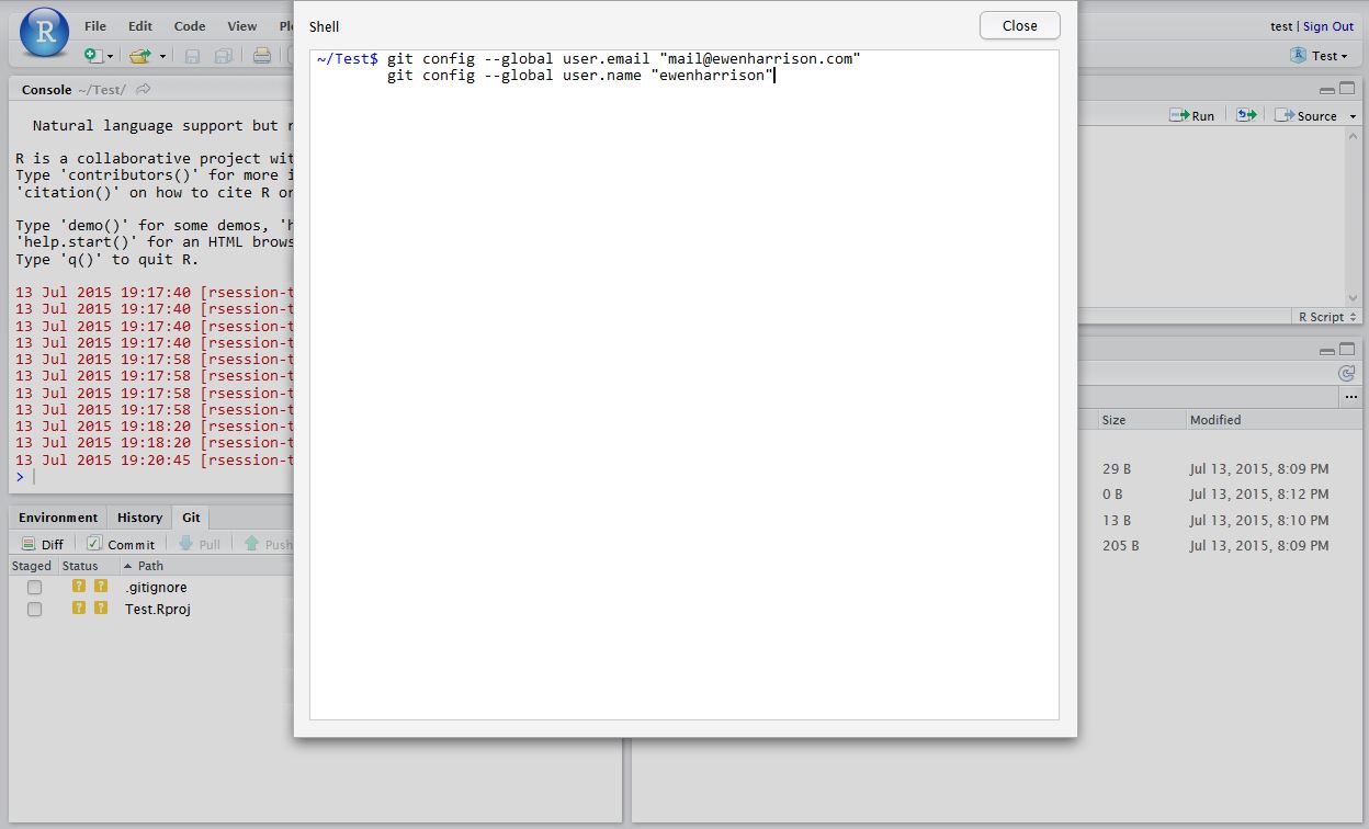
 Tell Git who you are. Remember Git is a piece of software running on your own computer. This is distinct to GitHub, which is the repository website. In RStudio, click Tools -> Shell … . Enter:
git config --global user.email "[email protected]"
git config --global user.name "ewenharrison"
Use your GitHub username.
Create New project AND git
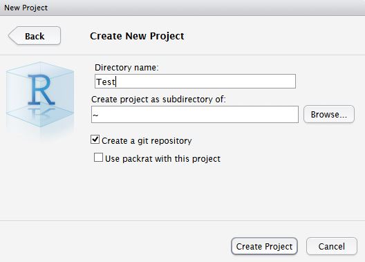
In RStudio, click New project as normal. Click New Directory.
Name the project and check Create a git repository.
Now in RStudio, create a new script which you will add to your repository.
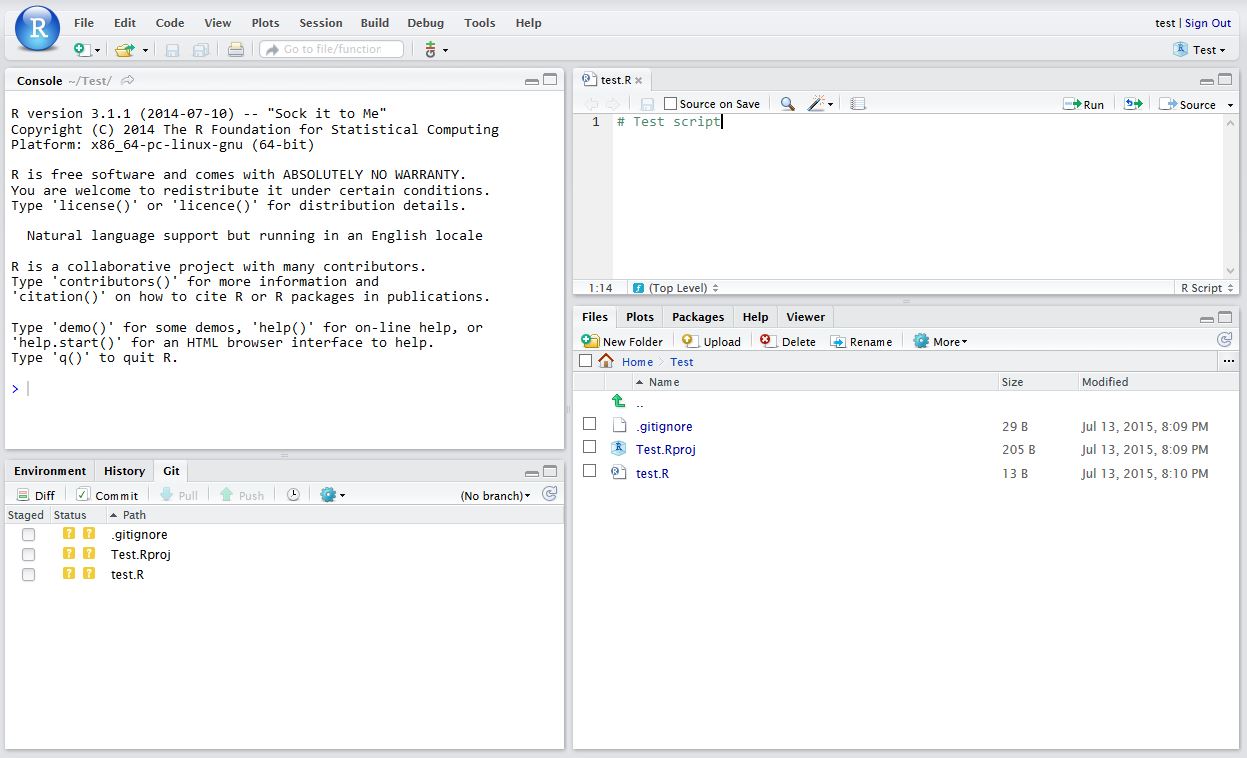 After saving your new script (test.R), it should appear in the Git tab on the Environment / history panel.
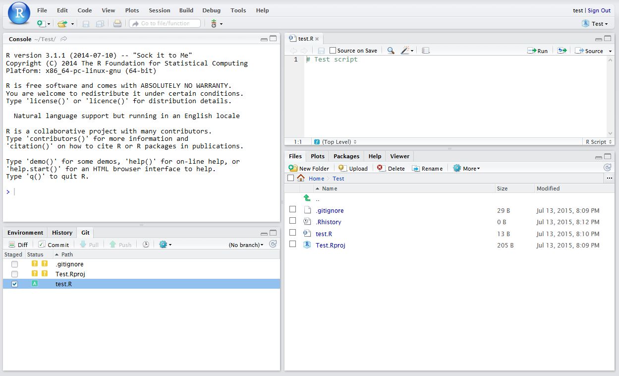 Click the file you wish to add, and the status should turn to a green ‘A’. Now click Commit and enter an identifying message in Commit message.
 You have now committed the current version of this file to your repository on your computer/server. In the future you may wish to create branches to organise your work and help when collaborating.
Now you want to push the contents of this commit to GitHub, so it is also backed-up off site and available to collaborators. In GitHub, create a New repository, called here test.
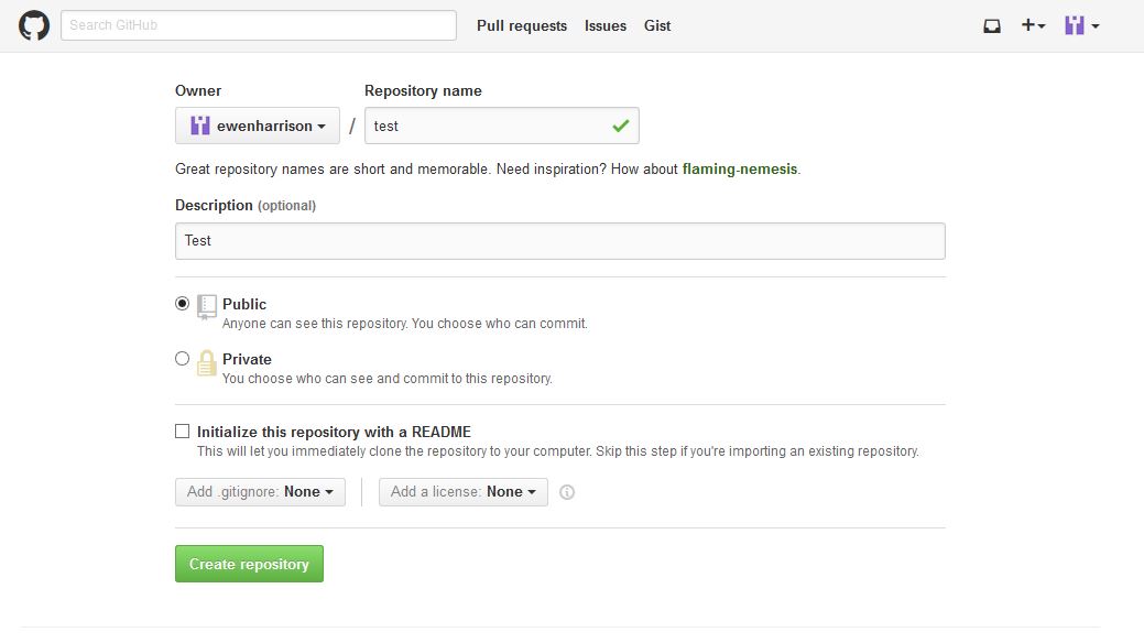 In RStudio, again click Tools -> Shell … . Enter:
git remote add origin https://github.com/ewenharrison/test.git
git config remote.origin.url [email protected]:ewenharrison/test.git
git pull -u origin master
git push -u origin master
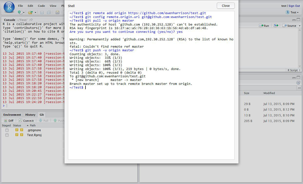 You have now pushed your commit to GitHub, and should be able to see your files in your GitHub account. The Pull Push buttons in RStudio will now also work. Remember, after each Commit, you have to Push to GitHub, this doesn’t happen automatically.
Clone an existing GitHub project to new RStudio project
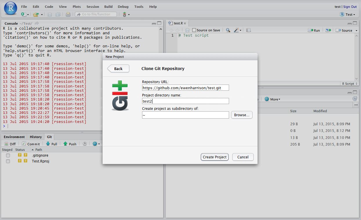
In RStudio, click New project as normal. Click Version Control.
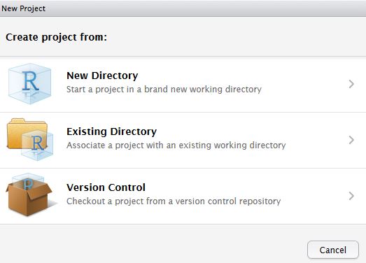 In Clone Git Repository, enter the GitHub repository URL as per below. Change the project directory name if necessary.
 In RStudio, again click Tools -> Shell … . Enter:
git config remote.origin.url [email protected]:ewenharrison/test.git
Interested in international trials? Take part in GlobalSurg.


