Here’s two handy scripts for hypothesis testing of summary data. I seem to use these a lot when checking work:
- Chi-squared test of association for categorical data.
- Student’s t-test for difference in means of normally distributed data.
The actual equations are straightforward, but get involved when group sizes and variance are not equal. Why do I use these a lot?!
I wrote about a study from Hungary in which the variability in the results seemed much lower than expected. We wondered whether the authors had made a mistake in saying they were showing the standard deviation (SD), when in fact they had presented the standard error of the mean (SEM).
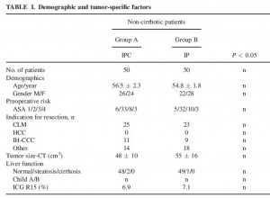
 This is a bit of table 1 from the paper. It shows the differences in baseline characteristics between the treated group (IPC) and the active control group (IP). In it, they report no difference between the groups for these characteristics, p>0.05.
But taking “age” as an example and using the simple script for a Student’s t-test with these figures, the answer we get is different. Mean (SD) for group A vs. group B: 56.5 (2.3) vs. 54.8 (1.8), t=4.12, df=98, p=<0.001.
There are lots of similar examples in the paper.
Using standard error of the mean rather than standard deviation gives a non-significant difference as expected.
$latex SEM=SD/\sqrt{n}.$
See here for how to get started with R.
####################
# Chi-sq test from #
# two by two table #
####################

#           Factor 1
# Factor 2  a   |   b
#           c   |   d

a<-32
b<-6
c<-43
d<-9

m<-rbind(c(a,b), c(c,d))
m
chisq.test(m, correct = FALSE)
# Details here
help(chisq.test)

############################
# T-test from summary data #
############################

# install.packages("BSDA") # remove first "#" to install first time only
library(BSDA)
x1<-56.5     # group 1 mean
x1_sd<-2.3   # group 1 standard deviation
n1<-50       # group 1 n
x2<-54.8     # group 2 mean
x2_sd<-1.8   # group 2 standard deviation
n2<-50       # group 2 n

tsum.test(x1, x1_sd, n1, x2, x2_sd, n2, var.equal = TRUE)
# Details here
help(tsum.test)


