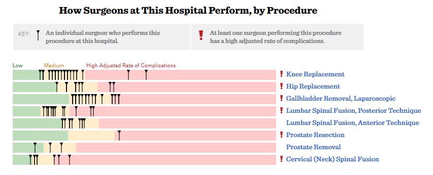
ProPublica, an independent investigative journalism organisation, have published surgeon-level complications rates based on Medicare data. I have already highlighted problems with the reporting of the data: surgeons are described as having a “high adjusted rate of complications” if they fall in the red-zone, despite there being too little data to say whether this has happened by chance.

I say again, I fully support transparency and public access to healthcare. But the ProPublica reporting has been quite shocking. I’m not aware of them publishing the number of surgeons out of the 17000 that are statistically different to the average. This is a small handful.
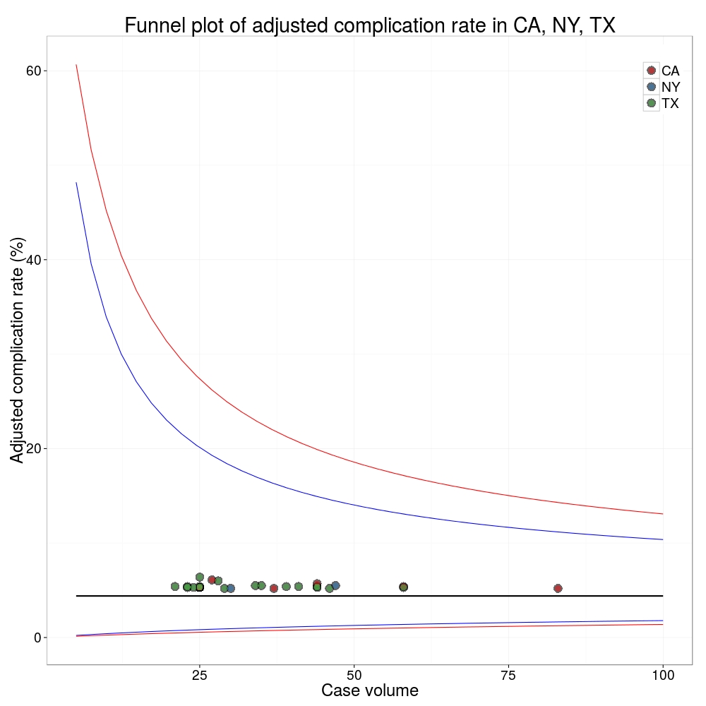
ProPublica could have chosen a different approach. This is a funnel plot and I’ve written about them before.
A funnel plot is a summary of an estimate (such as complication rate) against a measure of the precision of that estimate. In the context of healthcare, a centre or individual outcome is often plotted against patient volume. A horizontal line parallel to the x-axis represents the outcome for the entire population and outcomes for individual surgeons are displayed as points around this. This allows a comparison of individuals with that of the population average, while accounting for the increasing certainty surrounding that outcome as the sample size increases. Limits can be determined, beyond which the chances of getting an individual outcome are low if that individual were really part of the whole population.
In other words, a surgeon above the line has a complication rate different to the average.
I’ve scraped the ProPublica data for gallbladder removal (laparoscopic cholecystectomy) from California, New York and Texas for surgeons highlighted in the red-zone. These are surgeons ProPublica says have high complication rates.
As can be seen from the funnel plot, these surgeons are no where near being outliers. There is insufficient information to say whether any of them are different to average. ProPublica decided to ignore the imprecision with which the complication rates are determined. For red-zone surgeons from these 3 states, none of them have complication rates different to average.
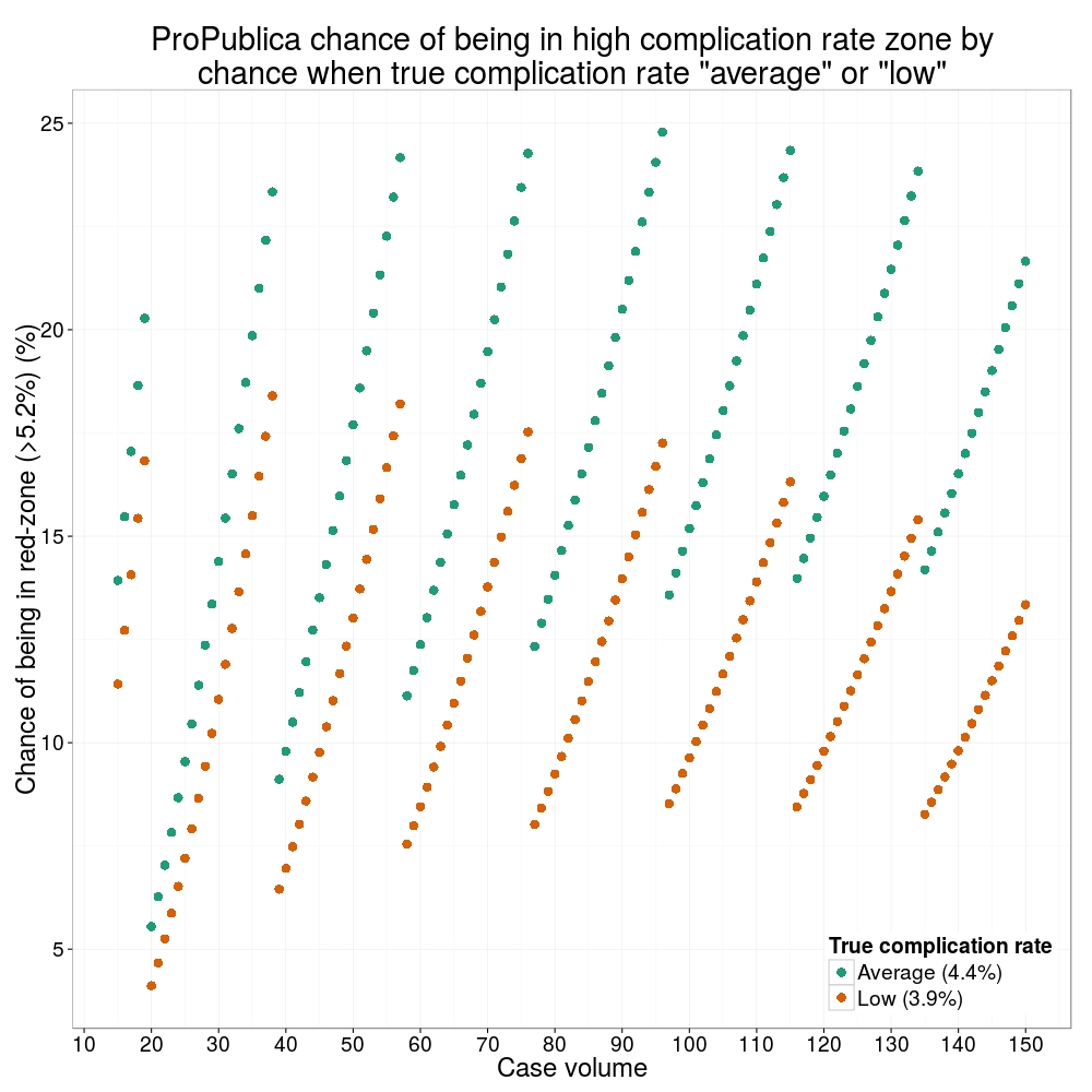
How likely is it that a surgeon with an average complication rate (4.4%) will appear in the red-zone just by chance (>5.2%)? The answer is, pretty likely given the small numbers of cases here: anything up to a 25% chance depending on the number of cases performed. Even at the top of the green-zone (low ACR, 3.9%), there is still around a 1 in 6 chance a surgeon will appear to have a high complication rate just by chance.
 ProPublica have failed in their duty to explain these data in a way that can be understood. The surgeon score card should be revised. All “warning explanation points” should be removed for those other than the truly outlying cases.
Data
Git
Code
# ProPublica Surgeon Scorecard
# https://projects.propublica.org/surgeons

# Laparoscopic cholecystectomy (gallbladder removal) data
# Surgeons with "high adjusted rate of complications"
# CA, NY, TX only

# Libraries needed ----
library(ggplot2)
library(binom)

# Upload dataframe ----
dat = read.csv("http://www.datasurg.net/wp-content/uploads/2015/07/ProPublica_CA_NY_TX.csv")

# Total number reported
dim(dat)[1] # 59

# Remove duplicate surgeons who operate in more than one hospital
duplicates = which(
    duplicated(dat$Surgeon)
)

dat_unique = dat[-duplicates,]
dim(dat_unique) # 27

# Funnel plot for gallbladder removal adjusted complication rate -------------------------
# Set up blank funnel plot ----
# Set control limits
pop.rate = 0.044 # Mean population ACR, 4.4%
binom_n = seq(5, 100, length.out=40)
ci.90 = binom.confint(pop.rate*binom_n, binom_n, conf.level = 0.90, methods = "wilson")
ci.95 = binom.confint(pop.rate*binom_n, binom_n, conf.level = 0.95, methods = "wilson")
ci.99 = binom.confint(pop.rate*binom_n, binom_n, conf.level = 0.99, methods = "wilson")

theme_set(theme_bw(24))
g1 = ggplot()+
    geom_line(data=ci.95, aes(ci.95$n, ci.95$lower*100), colour = "blue")+
    geom_line(data=ci.95, aes(ci.95$n, ci.95$upper*100), colour = "blue")+
    geom_line(data=ci.99, aes(ci.99$n, ci.99$lower*100), colour = "red")+
    geom_line(data=ci.99, aes(ci.99$n, ci.99$upper*100), colour = "red")+
    geom_line(aes(x=ci.90$n, y=pop.rate*100), colour="black", size=1)+
    xlab("Case volume")+
    ylab("Adjusted complication rate (%)")+
    scale_colour_brewer("", type = "qual", palette = 6)+
    theme(legend.justification=c(1,1), legend.position=c(1,1))
g1

g1 +
    geom_point(data=dat_unique, aes(x=Volume, y=ACR), colour="black", alpha=0.6, size = 6,
                         show_guide=TRUE)+
    geom_point(data=dat_unique, aes(x=Volume, y=ACR, colour=State), alpha=0.6, size=4) +
    ggtitle("Funnel plot of adjusted complication rate in CA, NY, TX")


# Probability of being shown as having high complication rate ----
# At 4.4%, what are the changes of being 5.2% by chance?
n <- seq(15, 150, 1)
average = 1-pbinom(ceiling(n*0.052), n, 0.044)
low = 1-pbinom(ceiling(n*0.052), n, 0.039)

dat_prob = data.frame(n, average, low)

ggplot(melt(dat_prob, id="n"))+
    geom_point(aes(x=n, y=value*100, colour=variable), size=4)+
    scale_x_continuous("Case volume", breaks=seq(10, 150, 10))+
    ylab("Adjusted complication rate (%)")+
    scale_colour_brewer("True complication rate", type="qual", palette = 2, labels=c("Average (4.4%)", "Low (3.9%)"))+
    ggtitle("ProPublica chance of being in high complication rate zone by\nchance when true complication rate \"average\" or \"low\"")+
    theme(legend.position=c(1,0), legend.justification=c(1,0))


