Riinu and I are sitting in Frankfurt airport discussing the paper retracted in JAMA this week.
During analysis, the treatment variable coded [1,2] was recoded in error to [1,0]. The results of the analysis were therefore reversed. The lung-disease self-management program actually resulted in more attendances at hospital, rather than fewer as had been originally reported.
Recode check
Checking of recoding is such an important part of data cleaning – we emphasise this a lot in HealthyR courses – but of course mistakes happen.
Our standard approach is this:
library(finalfit)
colon_s %>%
  mutate(
    sex.factor2 = forcats::fct_recode(sex.factor,
      "F" = "Male",
      "M" = "Female")
  ) %>%
  count(sex.factor, sex.factor2)
# A tibble: 2 x 3
  sex.factor sex.factor2     n
  <fct>      <fct>       <int>
1 Female     M             445
2 Male       F             484
The miscode should be obvious.
check_recode()
However, mistakes may still happen and be missed. So we’ve bashed out a useful function that can be applied to your whole dataset. This is not to replace careful checking, but may catch something that has been missed.
The function takes a data frame or tibble and fuzzy matches variable names. It produces crosstables similar to above for all matched variables.
So if you have coded something from `sex` to `sex.factor` it will be matched. The match is hungry so it is more likely to match unrelated variables than to miss similar variables. But if you recode `death` to `mortality` it won’t be matched.
Here’s a walk through.
# Install
devtools::install_github('ewenharrison/finalfit')
library(finalfit)
library(dplyr)
# Recode example
colon_s_small = colon_s %>%
  select(-id, -rx, -rx.factor) %>%
  mutate(
    age.factor2 = forcats::fct_collapse(age.factor,
      "<60 years" = c("<40 years", "40-59 years")),
    sex.factor2 = forcats::fct_recode(sex.factor,
    # Intentional miscode
      "F" = "Male",
      "M" = "Female")
  )
# Check
colon_s_small %>%
  check_recode()
$index
# A tibble: 3 x 2
  var1        var2
  <chr>       <chr>
1 sex.factor  sex.factor2
2 age.factor  age.factor2
3 sex.factor2 age.factor2
$counts
$counts[[1]]
# A tibble: 2 x 3
  sex.factor sex.factor2     n
  <fct>      <fct>       <int>
1 Female     M             445
2 Male       F             484
$counts[[2]]
# A tibble: 3 x 3
  age.factor  age.factor2     n
  <fct>       <fct>       <int>
1 <40 years   <60 years      70
2 40-59 years <60 years     344
3 60+ years   60+ years     515
$counts[[3]]
# A tibble: 4 x 3
  sex.factor2 age.factor2     n
  <fct>       <fct>       <int>
1 M           <60 years     204
2 M           60+ years     241
3 F           <60 years     210
4 F           60+ years     274
As can be seen, the output takes the form of a list length 2. The first is an index of matched variables. The second is crosstables as tibbles for each variable combination. sex.factor2 can be seen as being miscoded. sex.factor2 and age.factor2 have been matched, but should be ignored.
Numerics are not included by default. To do so:
out = colon_s_small %>%
  select(-extent, -extent.factor,-time, -time.years) %>% # choose to exclude variables
  check_recode(include_numerics = TRUE)
out
# Output not printed for space
Miscoding in survival::colon dataset?
When doing this just today, we noticed something strange in our example dataset, survival::colon.
The variable node4 should be a binary recode of nodes greater than 4. But as can be seen, something is not right!
We’re interested in any explanations those working with this dataset might have.
There we are then, a function that may be useful in detecting miscoding. So useful in fact, that we have immediately found probable miscoding in a standard R dataset.
We are using multiple imputation more frequently to “fill in” missing data in clinical datasets. Multiple datasets are created, models run, and results pooled so conclusions can be drawn.
We’ve put some improvements into Finalfit on GitHub to make it easier to use with the mice package. These will go to CRAN soon but not immediately.
Multivariate Imputation by Chained Equations (mice)
miceis a great package and contains lots of useful functions for diagnosing and working with missing data. The purpose here is to demonstrate how mice can be integrated into the Finalfit workflow with inclusion of model from imputed datasets in tables and plots.
Choose variables to impute and variables to impute from
finalfit::missing_predictorMatrix()makes it easy to specify which variables do what. For instance, we often do not want to impute our outcome or explanatory variable of interest (exposure), but do want to use them to impute other variables.
This is straightforward to code using the arguments drop_from_imputed and drop_from_imputer.
library(mice)

# Specify model
explanatory = c("age", "sex.factor", "nodes",
  "obstruct.factor", "smoking_mar")
dependent = "mort_5yr"

# Choose not to impute missing values
# for explanatory variable of interest and
# outcome variable.
# But include in algorithm for imputation.
predM = colon_s %>%
	select(dependent, explanatory) %>%
	missing_predictorMatrix(
		drop_from_imputed = c("obstruct.factor", "mort_5yr")
	)
Create imputed datasets
A set of multiple imputed datasets (mids) can be created as below. Various checks should be performed to ensure you understand the data that has been created. See here.
mids = colon_s %>%
  select(dependent, explanatory) %>%
  mice(m = 4, predictorMatrix = predM)    # Usually m = 10
Run models
Here we sill use a logistic regression model. The with.mids() function takes a model with a formula object, so use base R functions rather than Finalfit wrappers.
We now have multiple models run with each of the imputed datasets. We haven’t found good methods for combining common model metrics like AIC and c-statistic. I’d be interested to hear from anyone working on methods for this. Metrics can be extracted for each individual model to give an idea of goodness-of-fit and discrimination. We’re not suggesting you use these to compare imputed datasets, but could use them to compare models containing different variables created using the imputed datasets, e.g.
fits %>%
  getfit() %>%
  purrr::map(AIC)
[[1]]
[1] 1192.57

[[2]]
[1] 1191.09

[[3]]
[1] 1195.49

[[4]]
[1] 1193.729

# C-statistic
fits %>%
  getfit() %>%
  purrr::map(~ pROC::roc(.x$y, .x$fitted)$auc)
[[1]]
Area under the curve: 0.6839

[[2]]
Area under the curve: 0.6818

[[3]]
Area under the curve: 0.6789

[[4]]
Area under the curve: 0.6836
Pool results
Rubin’s rules are used to combine results of multiple models.
# Pool  results
fits_pool = fits %>%
  pool()
Plot results
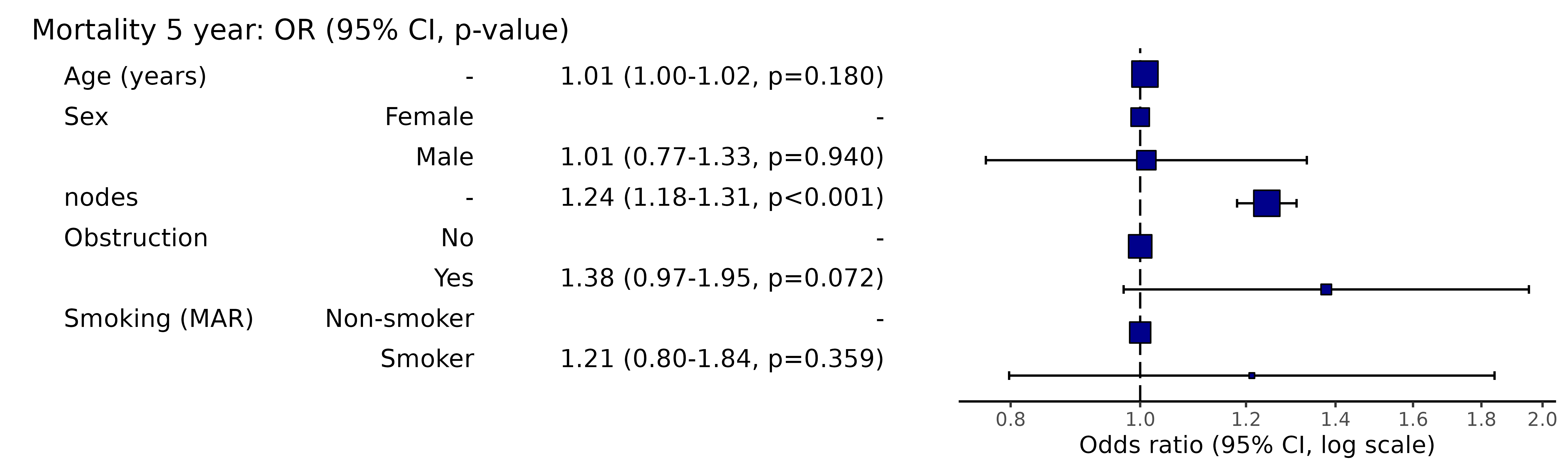
Pooled results can be passed directly to Finalfit plotting functions.
# Can be passed to or_plot
colon_s %>%
  or_plot(dependent, explanatory, glmfit = fits_pool, table_text_size=4)
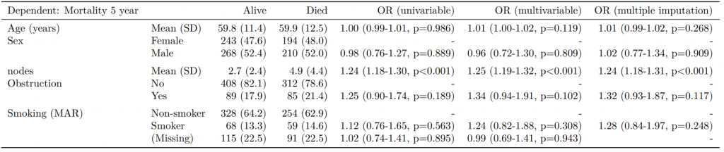
Put results in table
The pooled result can be passed directly to fit2df() as can many common models such as lm(), glm(), lmer(), glmer(), coxph(), crr(), etc.
# Summarise and put in table
fit_imputed = fits_pool %>%
  fit2df(estimate_name = "OR (multiple imputation)", exp = TRUE)
fit_imputed

         explanatory  OR (multiple imputation)
1                age 1.01 (1.00-1.02, p=0.212)
2     sex.factorMale 1.01 (0.77-1.34, p=0.917)
3              nodes 1.24 (1.18-1.31, p<0.001)
4 obstruct.factorYes 1.34 (0.94-1.91, p=0.105)
5  smoking_marSmoker 1.28 (0.88-1.85, p=0.192)
Combine results with summary data
Any model passed through fit2df() can be combined with a summary table generated with summary_factorlist() and any number of other models.
In healthcare, we deal with a lot of binary outcomes. Death yes/no, disease recurrence yes/no, for instance. These outcomes are often easily analysed using binary logistic regression via finalfit().
When the time taken for the outcome to occur is important, we need a different approach. For instance, in patients with cancer, the time taken until recurrence of the cancer is often just as important as the fact it has recurred.
Finalfit wraps a number of functions to make these analyses easy to perform and output into PDFs and Word documents.
Installation
# Make sure finalfit is up-to-date
install.packages("finalfit")
Dataset
We’ll use the classic “Survival from Malignant Melanoma” dataset from the boot package to illustrate. The data consist of measurements made on patients with malignant melanoma. Each patient had their tumour removed by surgery at the Department of Plastic Surgery, University Hospital of Odense, Denmark during the period 1962 to 1977.
For the purposes of demonstration, we are interested in the association between tumour ulceration and survival after surgery.
Get data and check
library(finalfit)
melanoma = boot::melanoma #F1 here for help page with data dictionary
ff_glimpse(melanoma)
#> Continuous
#>               label var_type   n missing_n missing_percent   mean     sd
#> time           time    <dbl> 205         0             0.0 2152.8 1122.1
#> status       status    <dbl> 205         0             0.0    1.8    0.6
#> sex             sex    <dbl> 205         0             0.0    0.4    0.5
#> age             age    <dbl> 205         0             0.0   52.5   16.7
#> year           year    <dbl> 205         0             0.0 1969.9    2.6
#> thickness thickness    <dbl> 205         0             0.0    2.9    3.0
#> ulcer         ulcer    <dbl> 205         0             0.0    0.4    0.5
#>              min quartile_25 median quartile_75    max
#> time        10.0      1525.0 2005.0      3042.0 5565.0
#> status       1.0         1.0    2.0         2.0    3.0
#> sex          0.0         0.0    0.0         1.0    1.0
#> age          4.0        42.0   54.0        65.0   95.0
#> year      1962.0      1968.0 1970.0      1972.0 1977.0
#> thickness    0.1         1.0    1.9         3.6   17.4
#> ulcer        0.0         0.0    0.0         1.0    1.0
#>
#> Categorical
#> data frame with 0 columns and 205 rows
As can be seen, all variables are coded as numeric and some need recoding to factors.
Death status
status is the the patients status at the end of the study.
1 indicates that they had died from melanoma;
2 indicates that they were still alive and;
3 indicates that they had died from causes unrelated to their melanoma.
Competing risks: comparing 2 (alive) with 1 (died melanoma) accounting for 3 (died other); see more below.
Time and censoring
time is the number of days from surgery until either the occurrence of the event (death) or the last time the patient was known to be alive. For instance, if a patient had surgery and was seen to be well in a clinic 30 days later, but there had been no contact since, then the patient’s status would be considered 30 days. This patient is censored from the analysis at day 30, an important feature of time-to-event analyses.
Recode
library(dplyr)
library(forcats)
melanoma = melanoma %>%
  mutate(
    # Overall survival
    status_os = case_when(
      status == 2 ~ 0, # "still alive"
      TRUE ~ 1), # "died melanoma" or "died other causes"

    # Diease-specific survival
    status_dss = case_when(
      status == 2 ~ 0,  # "still alive"
      status == 1 ~ 1,  # "died of melanoma"
      status == 3 ~ 0), # "died of other causes is censored"

    # Competing risks regression
    status_crr = case_when(
    	status == 2 ~ 0,  # "still alive"
        status == 1 ~ 1,  # "died of melanoma"
        status == 3 ~ 2), # "died of other causes"

    # Label and recode other variables
    age = ff_label(age, "Age (years)"), # table friendly labels
    thickness = ff_label(thickness, "Tumour thickness (mm)"),
    sex = factor(sex) %>%
      fct_recode("Male" = "1",
                 "Female" = "0") %>%
      ff_label("Sex"),
    ulcer = factor(ulcer) %>%
      fct_recode("No" = "0",
                 "Yes" = "1") %>%
      ff_label("Ulcerated tumour")
  )
Kaplan-Meier survival estimator
We can use the excellent survival package to produce the Kaplan-Meier (KM) survival estimator. This is a non-parametric statistic used to estimate the survival function from time-to-event data. Note use of %$% to expose left-side of pipe to older-style R functions on right-hand side.
library(survival)

survival_object = melanoma %$%
  Surv(time, status_os)

# Explore:
head(survival_object) # + marks censoring, in this case "Alive"
#> [1]  10   30   35+  99  185  204

# Expressing time in years
survival_object = melanoma %$%
  Surv(time/365, status_os)
KM analysis for whole cohort
Model
The survival object is the first step to performing univariable and multivariable survival analyses.
If you want to plot survival stratified by a single grouping variable, you can substitute “survival_object ~ 1” by “survival_object ~ factor”
# Overall survival in whole cohort
my_survfit = survfit(survival_object ~ 1, data = melanoma)
my_survfit # 205 patients, 71 events
#> Call: survfit(formula = survival_object ~ 1, data = melanoma)
#>
#>       n  events  median 0.95LCL 0.95UCL
#>  205.00   71.00      NA    9.15      NA
Life table
A life table is the tabular form of a KM plot, which you may be familiar with. It shows survival as a proportion, together with confidence limits. The whole table is shown with summary(my_survfit).
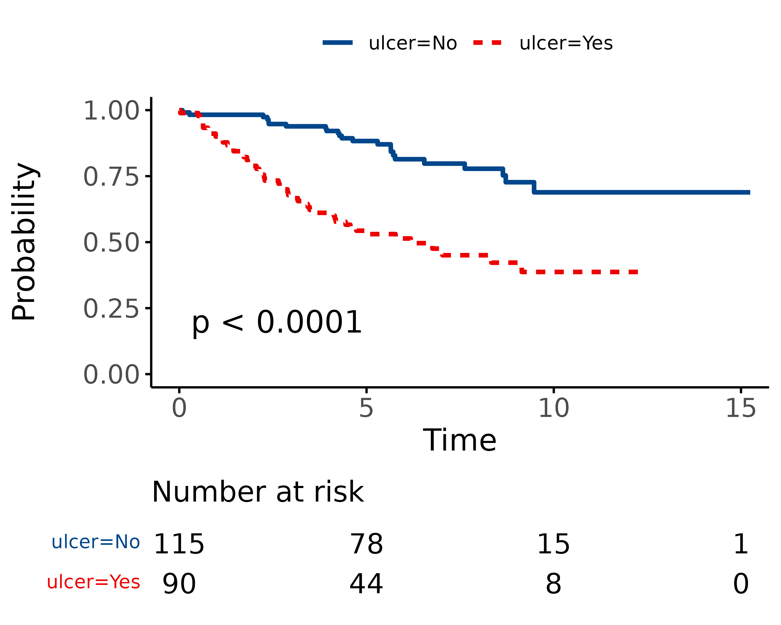
We can plot survival curves using the finalfit wrapper for the package excellent package survminer. There are numerous options available on the help page. You should always include a number-at-risk table under these plots as it is essential for interpretation.
As can be seen, the probability of dying is much greater if the tumour was ulcerated, compared to those that were not ulcerated.
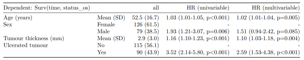
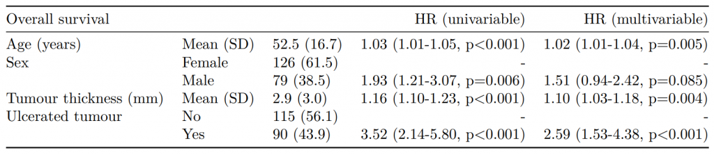
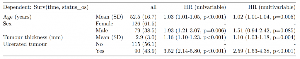
CPH regression can be performed using the all-in-one finalfit() function. It produces a table containing counts (proportions) for factors, mean (SD) for continuous variables and a univariable and multivariable CPH regression.
A hazard is the term given to the rate at which events happen.
The probability that an event will happen over a period of time is the hazard multiplied by the time interval.
An assumption of CPH is that hazards are constant over time (see below).
It produces a table containing counts (proportions) for factors, mean (SD) for continuous variables and a univariable and multivariable CPH regression.
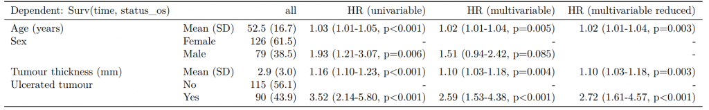
If you are using a backwards selection approach or similar, a reduced model can be directly specified and compared. The full model can be kept or dropped.
An assumption of CPH regression is that the hazard associated with a particular variable does not change over time. For example, is the magnitude of the increase in risk of death associated with tumour ulceration the same in the early post-operative period as it is in later years.
The cox.zph() function from the survival package allows us to test this assumption for each variable. The plot of scaled Schoenfeld residuals should be a horizontal line. The included hypothesis test identifies whether the gradient differs from zero for each variable. No variable significantly differs from zero at the 5% significance level.
zph_result
#>               rho  chisq      p
#> age        0.1633 2.4544 0.1172
#> sexMale   -0.0781 0.4473 0.5036
#> thickness -0.1493 1.3492 0.2454
#> ulcerYes  -0.2044 2.8256 0.0928
#> year       0.0195 0.0284 0.8663
#> GLOBAL         NA 8.4695 0.1322
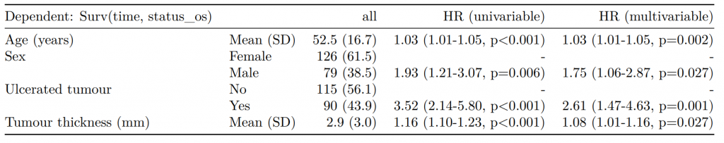
Stratified models
One approach to dealing with a violation of the proportional hazards assumption is to stratify by that variable. Including a strata() term will result in a separate baseline hazard function being fit for each level in the stratification variable. It will be no longer possible to make direct inference on the effect associated with that variable.
This can be incorporated directly into the explanatory variable list.
As a general rule, you should always try to account for any higher structure in the data within the model. For instance, patients may be clustered within particular hospitals.
There are two broad approaches to dealing with correlated groups of observations.
Including a cluster() term is akin to using generalised estimating equations (GEE). Here, a standard CPH model is fitted but the standard errors of the estimated hazard ratios are adjusted to account for correlations.
Including a frailty() term is akin to using a mixed effects model, where specific random effects term(s) are directly incorporated into the model.
Both approaches achieve the same goal in different ways. Volumes have been written on GEE vs mixed effects models. We favour the latter approach because of its flexibility and our preference for mixed effects modelling in generalised linear modelling. Note cluster() and frailty() terms cannot be combined in the same model.
The frailty() method here is being superseded by the coxme package, and we’ll incorporate this soon.
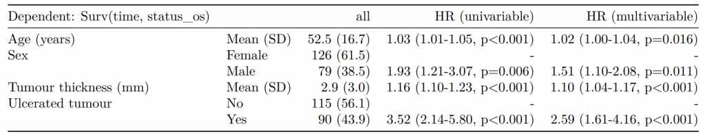
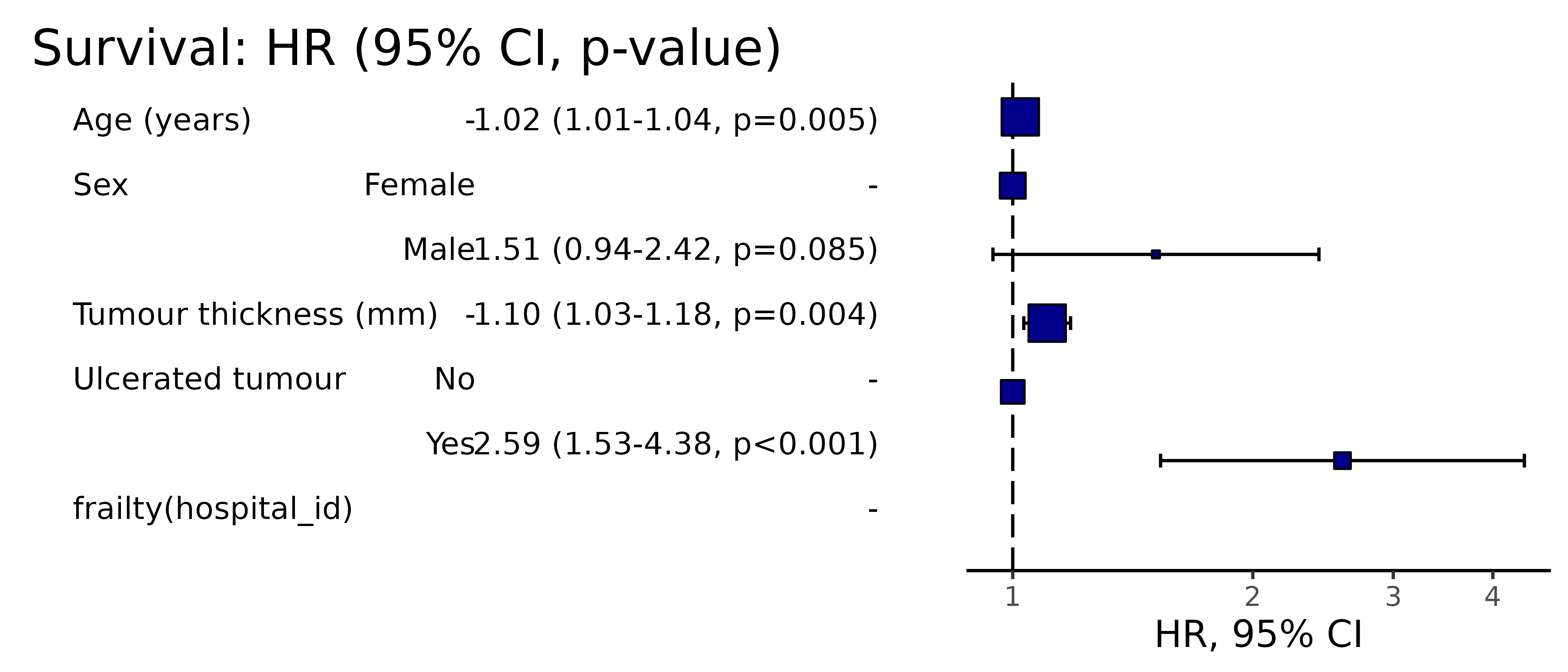
Hazard ratio plot
A plot of any of the above models can be produced by passing the terms to hr_plot().
melanoma %>%
    hr_plot(dependent_os, explanatory)
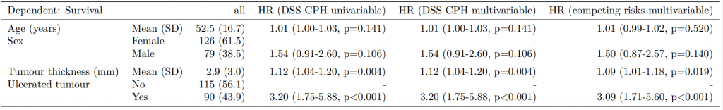
Competing risks regression
Competing-risks regression is an alternative to CPH regression. It can be useful if the outcome of interest may not be able to occur because something else (like death) has happened first. For instance, in our example it is obviously not possible for a patient to die from melanoma if they have died from another disease first. By simply looking at cause-specific mortality (deaths from melanoma) and considering other deaths as censored, bias may result in estimates of the influence of predictors.
The approach by Fine and Gray is one option for dealing with this. It is implemented in the package cmprsk. The crr() syntax differs from survival::coxph() but finalfit brings these together.
It uses the finalfit::ff_merge() function, which can join any number of models together.
So here we have various aspects of time-to-event analysis commonly used when looking at survival. There are many other applications, some which may not be obvious: for instance we use CPH for modelling length of stay in in hospital.
Stratification can be used to deal with non-proportional hazards in a particular variable.
Hierarchical structure in your data can be accommodated with cluster or frailty (random effects) terms.
Competing risks regression may be useful if your outcome is in competition with another, such as all-cause death, but is currently limited in its ability to accommodate hierarchical structures.
This blog is intended for researchers, PhD students, MD students and any other students who wish to have a robust and effective reference management setup. The blog has a particular focus on those using R markdown, Bookdown or LaTeX. Parts of the blog can also help setup Zotero for use with Microsoft Word. The blog has been designed to help achieve the following goals:
Effective citation storage
Fast and easy citation storage (one-click from Chrome)
Fast and easy PDF storage using cloud storage
Immediate, automatic and standardised PDF renaming
Immediate, automatic and standardised citation key generation
Effective citation integration with markdown etc.
Generation of citation keys which work with LaTeX and md (no non-standard characters)
Ability to lock citation keys so that they don’t update with Zotero updates
Storage of immediately updated .bib files for use with Rmd, Bookdown and LaTeX
Automated update of the .bib file in RStudio server
Downloads and Setup
For my current reference management setup I need the following software:
Zotfile is a Zotero plugin which helps with PDF management, download the .xpi file and then open Zotero, go to “Tools → Add-Ons” and click the little cog in the top right corner and navigate to file to install (Figure 1)
Better BibTeX is a plugin to help generate citation keys which will be essential for writing articles in LaTeX, R Markdown or Bookdown
If the link doesn’t work go to github and scroll down to the ReadMe to find a link to download the .xpi file
The same approach is then used to install the Better BibTeX plugin for zotero (“Tools → Add-Ons”)
Figure 1: Zotero Plugin/Add-on Installation
After downloading Zotero, ZotFile and Better BibTeX create an account on Zotero online.
In addition to the Zotero downloads this guide will focus on an efficient setup for writing with R markdown or Bookdown and assumes that you have access to the following software / accounts:
Dropbox / Google Drive / other cloud storage service which allows APIs
It will also be necessary for these to be accessible using Windows Explorer or Mac Finder (there are many guides online for syncing Google Drive and Dropbox so that they appear in file explorers)
RStudio (this is not 100% essential but it is far harder to use Rmd without it)
Packages which will be required for this setup include rdrop2 (if using dropbox, other packages are available to convert this setup to Google Drive etc.), encryptr, bookdown or Rmarkdown, tinytex and a LaTeX installation (the Bookdown author recommends using tinytex which can be installed by the similarly named R package: tinytex::install_tinytex())
Folder Setup
When using Zotero it is a good ideal to create a folder in which you will store PDFs retrieved from articles. Ultimately it is optional whether or not PDFs are stored but if you have access to cloud storage with a good quota then it can make writing in Rmd etc. much faster as there is no requirement to search online for the original PDF. This folder should be set up in Google Drive, Dropbox or another cloud storage service which can be accessed from your own computer through the file explorer.
A second folder may be useful to store bibliographies which will be generated for specific projects or submissions. Again this folder should be made available in cloud storage.
ZotFile Preferences
To setup Zotero so that retrieved PDFs are automatically stored and renamed in the cloud storage without consuming the Zotero storage quota go to “Tools → ZotFile Preferences” and on the first tab: General Settings and set the folder and subfolder naming strategy for PDFs. I have set the location of the files to a Custom location and in this case used the path to a Google Drive folder (~\Google Drive\Zotero PDF Library). ZotFile will also store retrieved PDFs in subfolders to help with finding PDFs at a later date. The current setup I use is to create a subfolder with the first author surname so that all papers authored by one (or more) author with the same name are stored together using the \%a in the subfolder field (Figure 2). Other alternatives are to store PDFs in subfolders using year (\%y); journal or publisher (\%w); or item type (\%T).
Figure 2: ZotFile Preferences
Next the Renaming Rules tab can be configured to provide sensible names to each of the files (this is essential if PDFs are not to be stored as random strings of characters which provide no meaning). In this tab I have set the format to: {%a_}{%y_}{%t} which provides names for the PDFs in the format of: Fairfield_2019_Gallstone_Disease_and_the_Risk_of_Cardiovascular_Disease.pdf. I find that this shows author, year and first word of title without needing to expand the file name (Figure 3).
Figure 3: ZotFile PDF Renaming Preferences
I have not changed any of the default settings in either the Tablet Settings or Advanved Settings tabs apart from removing special characters in the Advanced Settings (this stops things from breaking later).
General Zotero Settings
Zotero has several configurable settings (accessed through: “Edit → Preferences”) and I have either adopted the defaults or made changes as follows:
General:
I have ticked the following:
Automatically attach associated PDFs
Automatically retrieve metadata for PDFs
Automatically rename attachments using parent metadata
Automatically tag items with keywords and subject headings
All options in Group section
I have left the following unticked:
Automatically take snapshots
Rename linked files
Sync:
Enter the account details
Tick sync automatically
Untick sync full text (if you choose to save PDFs then syncing full text will quickly consume the 300MB quota)
Search:
Left unchanged
Export:
Left unchanged
Cite:
There are several sensible defaults but if there is a new citation style you wish to be able to use in Microsoft Word for example then click “Get additional styles” as there is probably a version that you need already created. You can click the “+” button to add a style from a .csl file if you have one already. Finally, if you are desperate for a style that doesn’t already exist then you can select a citation style and click Style Editor and edit the raw .csl file.
In the Word Processors subtab (on the main Cite tab), you can install the Microsoft Word add-in to allow Zotero to work in Microsoft Word.
Advanced:
I changed nothing on the General subtab
In the Files and Folders subtab I have selected the path to base directory for attachments
I have not changed the Shortcuts subtab
I have not changed the Feeds subtab
Better BibTex:
In this section I have set my Citation Key format to [auth:lower:alphanum]_[year:alphanum]_[veryshorttitle:lower:alphanum]_[journal:lower:clean:alphanum] (Figure 4). This generates a citation key for each reference in the format of fairfield_2019_gallstones_scientificreports or harrison_2012_hospital_bmj. It always takes the first author’s surname, the year, the first word of the title and the journal abbreviation if known. The clean and alphanum arguments to this field are used to remove unwanted punctuation which can cause citation to fail in LaTeX.
Figure 4: Better BibTeX Citation Key
Once the settings have been configured if you already had references stored in Zotero and wish to change the citation key for old references select your entire library root (above all folders), select all references, right click and use “Better BibTex → Refresh BibTeX Key” and all of the citation keys should be updated.
Creating a .bib file
For referencing in a new project, publication or submission it may be helpful to have a dynamic .bib file that updates with every new publication and can be accessed from any device through cloud storage.
To set up a .bib file, first find the folder that you wish to create the file from (this should be the folder which contains any citations you will use and ideally not the full library to cut down on unnecessary storage and syncing requirements). Note that the .bib file will generate a bibliography from any citations stored directly in the folder when using default settings. This prevents use of subfolders which I find particularly helpful for organising citations and I have therefore changed the setting so that folders also show any citations stored in subfolders. To make this change go to “Edit Preferences” and select the “Advanced” tab and at the bottom of the “General” subtab select “Config Editor”. This will bring up a searchable list of configurations (it may show a warning message before this) and search in the search box for “extensions.zotero.recursiveCollections”. Set “Value” to TRUE and then when you click a folder you should see all of the citations also stored in subfolders.
Right click the folder and select “Export Collection”. A pop-up window will appear at which point select “Keep Updated” and if using RStudio desktop save the file in the directory where you have your Rmd project files. If you are working with RStudio server then save the file in a cloud storage location which will then be accessed from the server. I have a .bib file stored in Dropbox which I access from RStudio server.
Linking Dropbox and RStudio Server to Access the .bib File
The following covers linking Dropbox to RStudio server but could be adapted to cover another cloud storage service.
Dropbox provides a token to allow communication between different apps. The rdrop2 package is what I used to create a token to allow this. I actually created the token on RStudio desktop as I couldn’t get the creation to work on the server but this is perfectly ok.
Caution: The token generated by this process could be used to access your Dropbox from anywhere using RStudio if you do not keep it secure. If somebody were to access an unencrypted token then it would be equivalent to handing out your email and password. I therefore used the encryptr package to allow safe storage of this token.
Token Creation
Open Rstudio desktop and enter the following code:
library(rdrop2)
library(encryptr)

# Create token
token <- drop_auth()

# Save token
saveRDS(token, "droptoken.rds")

# Encrypt token
genkeys()               # Default file names are id_rsa and id_rsa.pub
encrypt_file("droptoken.rds", "droptoken.rds.encryptr.bin")
encrypt_file(".httr-oauth", ".httr-oauth.encryptr.bin")

# Same details should appear later
drop_acc()

# Remove token from local environment
rm(token)


# Delete the unencrypted files
system("rm droptoken.rds")
system("rm .httr-oauth")
The code will create two files, a token and the .httr-oauth file from which a token can also be made. The encryptr package can then encrypt the files using a public / private key pair. It is essential that the password that is set when using genkeys() is remembered otherwise the token cannot then be used. In this case the original token can’t be retrieved but could be created again from scratch.
The following files will then be needed to upload to the RStudio server:
droptoken.rds.encryptr.bin – or the name provided for the encrypted Dropbox token
id_rsa – or the name provided for the private key from the private / public key pair
Dropbox Linkage for Referencing the .bib File
Now that the encrypted token and necessary (password-protected) private key are available in RStudio server, the following can be saved as a separate script. The script is designed to read in and decrypt the encrypted token (this will require a password and should be done if the .bib file needs updated). Only the drop_download() needs repeated if using the token again during the same session. The token should be cleared at the end of every session for additional security.
library(rdrop2)
library(encryptr)

# ******** WARNING ********
# Losing the unencrypted token will give anyone
# complete control of your Dropbox account
# If you are concerned this has happened,
# you can then revoke the rdrop2 app from your
# dropbox account and start over.
# ******** WARNING ********


safely_extract_dropbox_token <- function(encrypted_db_token = NULL, private_key_file = NULL){
  decrypt_file(encrypted_db_token, file_name = "temporary_dropbox_token.rds", private_key_path = private_key_file)

  token <<- readRDS("temporary_dropbox_token.rds")

  system("rm temporary_dropbox_token.rds")
}

safely_extract_dropbox_token(encrypted_db_token = "droptoken.rds.encryptr.bin", private_key_file = "id_rsa")

# Then pass the token to each drop_ function
drop_acc(dtoken = token)

# The path is the Dropbox file location
drop_download(path = "My_Dropbox_Home_Directory/Zotero Library/my.bib",
              local_path = "my.bib",
              dtoken = token,
              overwrite = TRUE)
Now that the .bib file has been created and is stored as “my.bib” in the local directory, it should update whenever the token is loaded and drop_download() is run.
Final Result
On clicking “Save to Zotero” button in Chrome and running drop_download() the following should all happen almost instantaneously:
Zotero stores a new reference
A PDF is stored in the cloud storage having been named appropriately
A link to the PDF is stored in Zotero (without using up significant memory)
A citation key is established for the reference in a standardised format without conflicts
Pre-existing citation keys which have been referenced earlier in the writing of the paper are not altered
A .bib file is updated in the RStudio server directory
And much unwanted frustration of reference management is resolved
This is my current reference management system which I have so far found to be very effective. If there are ways you think it can be improved I would love to hear about them.
Data security is paramount and encryptr was written to make this easier for non-experts. Columns of data can be encrypted with a couple of lines of R code, and single cells decrypted as required.
But what was missing was an easy way to encrypt the file source of that data.
Now files can be encrypted with a couple of lines of R code.
Encryption and decryption with asymmetric keys is computationally expensive. This is how encrypt for data columns works. This makes it easy for each piece of data in a data frame to be decrypted without compromise of the whole data frame. This works on the presumption that each cell contains less than 245 bytes of data.
File encryption requires a different approach as files are larger in size. encrypt_file encrypts a file using a symmetric “session” key and the AES-256 cipher. This key is itself then encrypted using a public key generated using genkeys. In OpenSSL this combination is referred to as an envelope.
It should work with any type of single file but not folders.
genkeys()
#> Private key written with name 'id_rsa'
#> Public key written with name 'id_rsa.pub'
Encrypt file
To demonstrate, the included dataset is written as a .csv file.
write.csv(gp, "gp.csv")
encrypt_file("gp.csv")
#> Encrypted file written with name 'gp.csv.encryptr.bin'
Important: check that the file can be decrypted prior to removing the original file from your system.
Warning: it is strongly suggested that the original unencrypted data file is securely stored else where as a back-up in case unencryption is not possible, e.g., the private key file or password is lost
Decrypt file
The decrypt_file function will not allow the original file to be overwritten, therefore if it is still present, use the option to specify a new name for the unencrypted file.
decrypt_file("gp.csv.encryptr.bin", file_name = "gp2.csv")
#> Decrypted file written with name 'gp2.csv'
Support / bugs
The new version 0.1.3 is on its way to CRAN today or you can install from github:
A number of existing R packages support data encryption. However, we haven’t found one that easily suits our needs: to encrypt one or many columns of a data frame or tibble using a private/public key pair in tidyverse functions. The emphasis is on the easily.
Encrypting and decrypting data securely is important when it comes to healthcare and sociodemographic data. We have developed a simple and secure package encryptyr which allows non-experts to encrypt and decrypt columns of data.
There is a simple and easy-to-follow vignette available on our GitHub page which guides you through the process of using encryptr:
Data containing columns of disclosive or confidential information such as a postcode or a patient ID (CHI in Scotland) require extreme care. Storing sensitive information as raw values leaves the data vulnerable to confidentiality breaches.
It is best to just remove confidential information from the records whenever possible. However, this can mean the data can never be re-associated with an individual. This may be a problem if, for example, auditors of a clinical trial need to re-identify an individual from the trial data.
One potential solution currently in common use is to generate a study number which is linked to the confidential data in a separate lookup table, but this still leaves the confidential data available in another file.
Encryptr package solution – storing encrypted data
The encryptr package allows users to store confidential data in a pseudoanonymised form, which is far less likely to result in re-identification.
The package allows users to create a public key and a private key to enable RSA encryption and decryption of the data. The public key allows encryption of the data. The private key is required to decrypt the data. The data cannot be decrypted with the public key. This is the basis of many modern encryption systems.
When creating keys, the user sets a password for the private key using a dialogue box. This means that the password is not included in an R script. We recommend creating a secure password with a variety of alphanumeric characters and symbols.
As the password is not stored, it is important that you are able to remember it if you need to decrypt the data later.
Once the keys are created it is possible to encrypt one or more columns of data in a data frame or tibble using the public key. Every time RSA encryption is used it will generate a unique output. Even if the same information is encrypted more than once, the output will always be different. It is not possible therefore to match two encrypted values.
These outputs are also secure from decryption without the private key. This may allow sharing of data within or between research teams without sharing confidential data.
Caution: data often remains potentially disclosive (or only pseudoanomymised) even after encryption of identifiable variables and all of the required permissions for usage and sharing of data must still be in place.
Encryptr package – decrypting the data
Sometimes decrypting data is necessary. For example, participants in a clinical trial may need to be contacted to explain a change or early termination of the trial.
The encryptr package allows users to securely and reliably decrypt the data. The decrypt function will use the private key to decrypt one or more columns. The user will be required to enter the password created when the keys were generated.
As the private key is able to decrypt all of the data, we do not recommend sharing this key.
Blinding and unblinding clinical trials – another encryptr package use
Often when working with clinical trial data, the participants are randomised to one or more treatment groups. Often teams working on the trial are unaware of the group to which patients were randomised (blinded).
Using the same method of encryption, it is possible to encrypt the participant allocation group, allowing the sharing of data without compromising blinding. If other members of the trial team are permitted to see treatment allocation (unblinded), then the decryption process can be followed to reveal the group allocation.
What this is not
This is a simple set of wrappers of openssl aimed at non-experts. It does not seek to replace the many excellent encryption packages available in R, such as PKI, sodium and safer. We believe however that it makes things much easier. Comments and forks welcome.
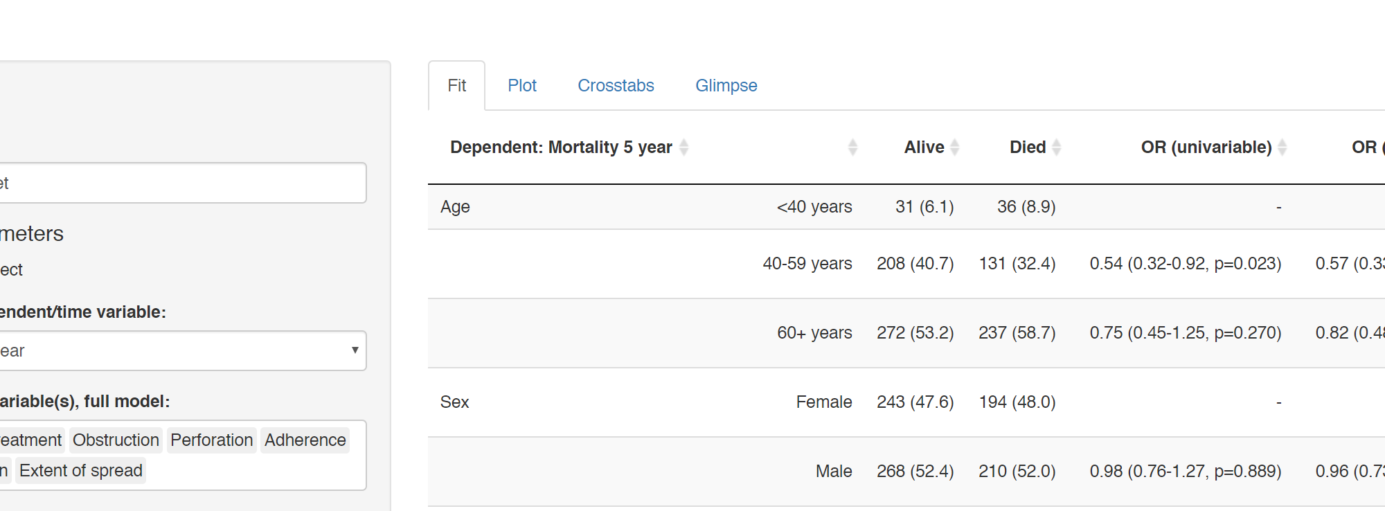
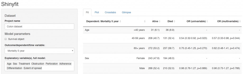
Many of our projects involve getting doctors, nurses, and medical students to collect data on the patients they are looking after. We want to involve many of them in data analysis, without the requirement for coding experience or access to statistical software. To achieve this we have built Shinyfit, a shiny app for linear, logistic, and Cox PH regression.
Aim: allow access to model fitting without requirement for statistical software or coding experience.
Audience: Those sharing datasets in context of collaborative research or teaching.
Hosting requirements: Basic R coding skills including tidyverse to prepare dataset (5-10 minutes).
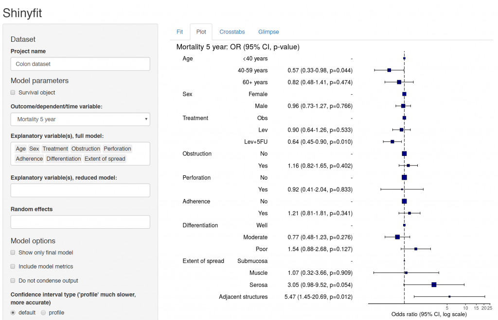
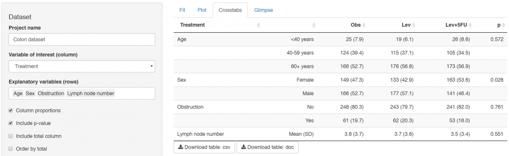
Linear, logistic or CPH regression tables Coefficient, odds ratio or hazard ratio plotsCrosstabsInspect dataset with ff_glimpse
Use your data
To use your own data, clone or download app from github.
Edit 0_prep.R to create a shinyfit_data object.
Test the app, usually within RStudio.
Deploy to your shiny hosting platform of choice.
Ensure you have permission to share the data
Editing 0_prep.R is straightforward and takes about 5 mins. The main purpose is to create human-readable menu items and allows sorting of variables into any categories, such as outcome and explanatory.
Errors in shinyfit are usually related to the underlying dataset, e.g.
Variables not appropriately specified as numerics or factors.
A particular factor level is empty, thus regression function (lm, glm, coxph etc.) gives error.
A variable with >2 factor levels is used as an outcome/dependent. This is not supported.
Use Glimpse tabs to check data when any error occurs.
It is fully mobile compliant, including datatables.
There will be bugs. Please report here.
As a journal editor, I often receive studies in which the investigators fail to describe, analyse, or even acknowledge missing data. This is frustrating, as it is often of the utmost importance. Conclusions may (and do) change when missing data is accounted for. A few seem to not even appreciate that in conventional regression, only rows with complete data are included.
These are the five steps to ensuring missing data are correctly identified and appropriately dealt with:
Ensure your data are coded correctly.
Identify missing values within each variable.
Look for patterns of missingness.
Check for associations between missing and observed data.
Decide how to handle missing data.
Finalfit includes a number of functions to help with this.
Some confusing terminology
But first there are some terms which easy to mix up. These are important as they describe the mechanism of missingness and this determines how you can handle the missing data.
Missing completely at random (MCAR)
As it says, values are randomly missing from your dataset. Missing data values do not relate to any other data in the dataset and there is no pattern to the actual values of the missing data themselves.
For instance, when smoking status is not recorded in a random subset of patients.
This is easy to handle, but unfortunately, data are almost never missing completely at random.
Missing at random (MAR)
This is confusing and would be better stated as missing conditionally at random. Here, missing data do have a relationship with other variables in the dataset. However, the actual values that are missing are random.
For example, smoking status is not documented in female patients because the doctor was too shy to ask. Yes ok, not that realistic!
Missing not at random (MNAR)
The pattern of missingness is related to other variables in the dataset, but in addition, the values of the missing data are not random.
For example, when smoking status is not recorded in patients admitted as an emergency, who are also more likely to have worse outcomes from surgery.
Missing not at random data are important, can alter your conclusions, and are the most difficult to diagnose and handle. They can only be detected by collecting and examining some of the missing data. This is often difficult or impossible to do.
How you deal with missing data is dependent on the type of missingness. Once you know this, then you can sort it.
More on this below.
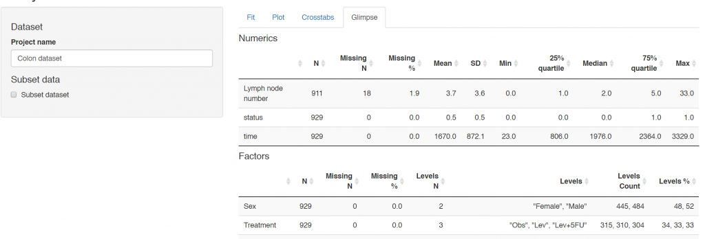
1. Ensure your data are coded correctly: ff_glimpse
While clearly obvious, this step is often ignored in the rush to get results. The first step in any analysis is robust data cleaning and coding. Lots of packages have a glimpse function and finalfit is no different. This function has three specific goals:
Ensure all factors and numerics are correctly assigned. That is the commonest reason to get an error with a finalfit function. You think you’re using a factor variable, but in fact it is incorrectly coded as a continuous numeric.
Ensure you know which variables have missing data. This presumes missing values are correctly assigned `NA`. See here for more details if you are unsure.
Ensure factor levels and variable labels are assigned correctly.
Example scenario
Using the colon cancer dataset that comes with finalfit, we are interested in exploring the association between a cancer obstructing the bowel and 5-year survival, accounting for other patient and disease characteristics.
For demonstration purposes, we will create random MCAR and MAR smoking variables to the dataset.
# Make sure finalfit is up-to-date
install.packages("finalfit")

library(finalfit)

# Create some extra missing data
## Smoking missing completely at random
set.seed(1)
colon_s$smoking_mcar =
  sample(c("Smoker", "Non-smoker", NA),
    dim(colon_s)[1], replace=TRUE,
    prob = c(0.2, 0.7, 0.1)) %>%
  factor()
Hmisc::label(colon_s$smoking_mcar) = "Smoking (MCAR)"

## Smoking missing conditional on patient sex
colon_s$smoking_mar[colon_s$sex.factor == "Female"] =
  sample(c("Smoker", "Non-smoker", NA),
    sum(colon_s$sex.factor == "Female"),
    replace = TRUE,
    prob = c(0.1, 0.5, 0.4))

colon_s$smoking_mar[colon_s$sex.factor == "Male"] =
  sample(c("Smoker", "Non-smoker", NA),
    sum(colon_s$sex.factor == "Male"),
    replace=TRUE, prob = c(0.15, 0.75, 0.1))
colon_s$smoking_mar = factor(colon_s$smoking_mar)
Hmisc::label(colon_s$smoking_mar) = "Smoking (MAR)"
The function summarises a data frame or tibble by numeric (continuous) variables and factor (discrete) variables. The dependent and explanatory are for convenience. Pass either or neither e.g. to summarise data frame or tibble:
colon %>%
  ff_glimpse()
It doesn’t present well if you have factors with lots of levels, so you may want to remove these.
Use this to check that the variables are all assigned and behaving as expected. The proportion of missing data can be seen, e.g. smoking_mar has 23% missing data.
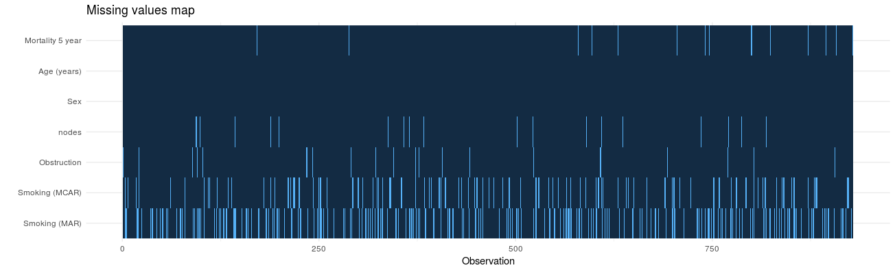
2. Identify missing values in each variable: missing_plot
In detecting patterns of missingness, this plot is useful. Row number is on the x-axis and all included variables are on the y-axis. Associations between missingness and observations can be easily seen, as can relationships of missingness between variables.
colon_s %>%
  missing_plot()
Click to enlarge.
It was only when writing this post that I discovered the amazing package, naniar. This package is recommended and provides lots of great visualisations for missing data.
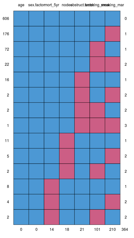
3. Look for patterns of missingness: missing_pattern
missing_pattern simply wraps mice::md.pattern using finalfit grammar. This produces a table and a plot showing the pattern of missingness between variables.
This allows us to look for patterns of missingness between variables. There are 14 patterns in this data. The number and pattern of missingness help us to determine the likelihood of it being random rather than systematic.
Make sure you include missing data in demographics tables
Table 1 in a healthcare study is often a demographics table of an “explanatory variable of interest” against other explanatory variables/confounders. Do not silently drop missing values in this table. It is easy to do this correctly with summary_factorlist. This function provides a useful summary of a dependent variable against explanatory variables. Despite its name, continuous variables are handled nicely.
na_include=TRUE ensures missing data from the explanatory variables (but not dependent) are included. Note that any p-values are generated across missing groups as well, so run a second time with na_include=FALSE if you wish a hypothesis test only over observed data.
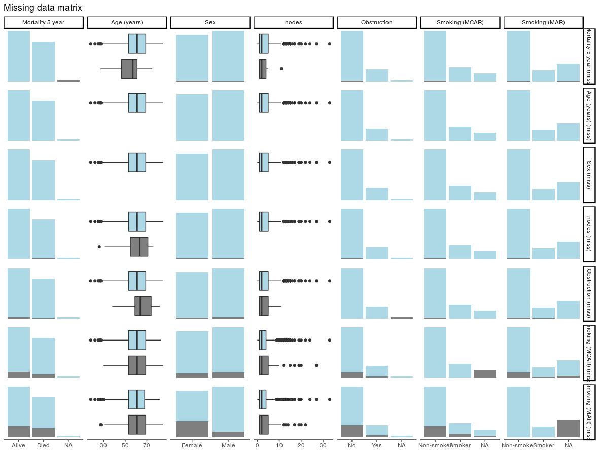
4. Check for associations between missing and observed data: missing_pairs | missing_compare
In deciding whether data is MCAR or MAR, one approach is to explore patterns of missingness between levels of included variables. This is particularly important (I would say absolutely required) for a primary outcome measure / dependent variable.
Take for example “death”. When that outcome is missing it is often for a particular reason. For example, perhaps patients undergoing emergency surgery were less likely to have complete records compared with those undergoing planned surgery. And of course, death is more likely after emergency surgery.
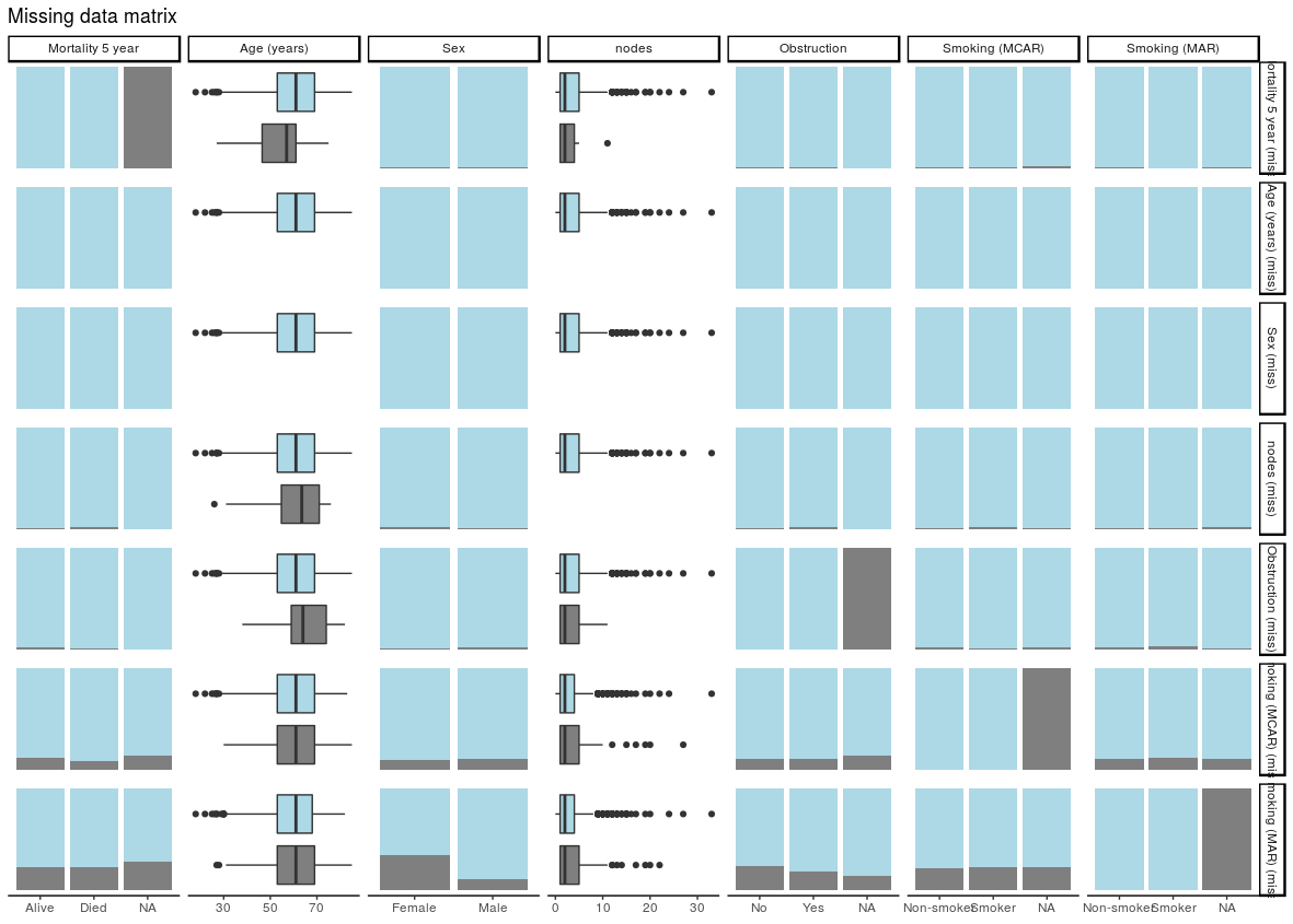
missing_pairs uses functions from the excellent GGally package. It produces pairs plots to show relationships between missing values and observed values in all variables.
For continuous variables (age and nodes), the distributions of observed and missing data can be visually compared. Is there a difference between age and mortality above?
For discrete, data, counts are presented by default. It is often easier to compare proportions:
colon_s %>%
  missing_pairs(dependent, explanatory, position = "fill", )
It should be obvious that missingness in Smoking (MCAR) does not relate to sex (row 6, column 3). But missingness in Smoking (MAR) does differ by sex (last row, column 3) as was designed above when the missing data were created.
We can confirm this using missing_compare.
explanatory = c("age", "sex.factor",
  "nodes", "obstruct.factor")
dependent = "smoking_mcar"
colon_s %>%
  missing_compare(dependent, explanatory)

 Missing data analysis: Smoking (MCAR)           Not missing     Missing     p
                           Age (years) Mean (SD) 59.7 (11.9) 59.9 (12.6) 0.867
                                   Sex    Female  399 (89.7)   46 (10.3) 0.616
                                            Male  429 (88.6)   55 (11.4)
                                 nodes Mean (SD)   3.6 (3.4)     4 (4.5) 0.990
                           Obstruction        No  654 (89.3)   78 (10.7) 0.786
                                             Yes  156 (88.6)   20 (11.4)

dependent = "smoking_mar"
colon_s %>%
  missing_compare(dependent, explanatory)

 Missing data analysis: Smoking (MAR)           Not missing    Missing      p
                          Age (years) Mean (SD) 59.6 (11.9)  60.1 (12)  0.709
                                  Sex    Female  288 (64.7) 157 (35.3) <0.001
                                           Male  431 (89.0)  53 (11.0)
                                nodes Mean (SD)   3.6 (3.6)  3.8 (3.6)  0.730
                          Obstruction        No  558 (76.2) 174 (23.8)  0.154
                                            Yes  143 (81.2)  33 (18.8)
It takes "dependent" and "explanatory" variables, but in this context "dependent" just refers to the variable being tested for missingness against the "explanatory" variables.
Comparisons for continuous data use a Kruskal Wallis and for discrete data a chi-squared test.
As expected, a relationship is seen between Sex and Smoking (MAR) but not Smoking (MCAR).
For those who like an omnibus test
If you are work predominately with numeric rather than discrete data (categorical/factors), you may find these tests from the MissMech package useful. The package and output is well documented, and provides two tests which can be used to determine whether data are MCAR.
These pages from Karen Grace-Martin are great for this.
Prior to a standard regression analysis, we can either:
Delete the variable with the missing data
Delete the cases with the missing data
Impute (fill in) the missing data
Model the missing data
MCAR, MAR, or MNAR
MCAR vs MAR
Using the examples, we identify that Smoking (MCAR) is missing completely at random.
We know nothing about the missing values themselves, but we know of no plausible reason that the values of the missing data, for say, people who died should be different to the values of the missing data for those who survived. The pattern of missingness is therefore not felt to be MNAR.
Common solution
Depending on the number of data points that are missing, we may have sufficient power with complete cases to examine the relationships of interest.
We therefore elect to simply omit the patients in whom smoking is missing. This is known as list-wise deletion and will be performed by default in standard regression analyses including finalfit.
explanatory = c("age", "sex.factor",
  "nodes", "obstruct.factor",
  "smoking_mcar")
dependent = "mort_5yr"
colon_s %>%
	finalfit(dependent, explanatory, metrics=TRUE)

 Dependent: Mortality 5 year                  Alive        Died          OR (univariable)        OR (multivariable)
                 Age (years)  Mean (SD) 59.8 (11.4) 59.9 (12.5) 1.00 (0.99-1.01, p=0.986) 1.01 (1.00-1.02, p=0.200)
                         Sex     Female  243 (47.6)  194 (48.0)                         -                         -
                                   Male  268 (52.4)  210 (52.0) 0.98 (0.76-1.27, p=0.889) 1.02 (0.76-1.38, p=0.872)
                       nodes  Mean (SD)   2.7 (2.4)   4.9 (4.4) 1.24 (1.18-1.30, p<0.001) 1.25 (1.18-1.33, p<0.001)
                 Obstruction         No  408 (82.1)  312 (78.6)                         -                         -
                                    Yes   89 (17.9)   85 (21.4) 1.25 (0.90-1.74, p=0.189) 1.53 (1.05-2.22, p=0.027)
              Smoking (MCAR) Non-smoker  358 (79.9)  277 (75.3)                         -                         -
                                 Smoker   90 (20.1)   91 (24.7) 1.31 (0.94-1.82, p=0.113) 1.37 (0.96-1.96, p=0.083)

"Number in dataframe = 929, Number in model = 782, Missing = 147, AIC = 1003.3, C-statistic = 0.687, H&L = Chi-sq(8) 15.03 (p=0.058)
Other considerations
Sensitivity analysis
Omit the variable
Imputation
Model the missing data
If the variable in question is thought to be particularly important, you may wish to perform a sensitivity analysis. A sensitivity analysis in this context aims to capture the effect of uncertainty on the conclusions drawn from the model. Thus, you may choose to re-label all missing smoking values as "smoker", and see if that changes the conclusions of your analysis. The same procedure can be performed labeling with "non-smoker".
If smoking is not associated with the explanatory variable of interest (bowel obstruction) or the outcome, it may be considered not to be a confounder and so could be omitted. That neatly deals with the missing data issue, but of course may not be appropriate.
Imputation and modelling are considered below.
MCAR vs MAR
But life is rarely that simple.
Consider that the smoking variable is more likely to be missing if the patient is female (missing_compareshows a relationship). But, say, that the missing values are not different from the observed values. Missingness is then MAR.
If we simply drop all the cases (patients) in which smoking is missing (list-wise deletion), then proportionality we drop more females than men. This may have consequences for our conclusions if sex is associated with our explanatory variable of interest or outcome.
Common solution
mice is our go to package for multiple imputation. That's the process of filling in missing data using a best-estimate from all the other data that exists. When first encountered, this doesn't sounds like a good idea.
However, taking our simple example, if missingness in smoking is predicted strongly by sex, and the values of the missing data are random, then we can impute (best-guess) the missing smoking values using sex and other variables in the dataset.
Imputation is not usually appropriate for the explanatory variable of interest or the outcome variable. With both of these, the hypothesis is that there is an meaningful association with other variables in the dataset, therefore it doesn't make sense to use these variables to impute them.
Here is some code to run mice. The package is well documented, and there are a number of checks and considerations that should be made to inform the imputation process. Read the documentation carefully prior to doing this yourself.
# Multivariate Imputation by Chained Equations (mice)
library(finalfit)
library(dplyr)
library(mice)
explanatory = c("age", "sex.factor",
  "nodes", "obstruct.factor", "smoking_mar")
dependent = "mort_5yr"

colon_s %>%
  select(dependent, explanatory) %>%
  # Exclude outcome and explanatory variable of interest from imputation
  dplyr::filter(!is.na(mort_5yr), !is.na(obstruct.factor)) %>%
  # Run imputation with 10 imputed sets
  mice(m = 10) %>%
  # Run logistic regression on each imputed set
  with(glm(formula(ff_formula(dependent, explanatory)),
    family="binomial")) %>%
  # Pool and summarise results
  pool() %>%
  summary(conf.int = TRUE, exponentiate = TRUE) %>%
  # Jiggle into finalfit format
  mutate(explanatory_name = rownames(.)) %>%
  select(explanatory_name, estimate, `2.5 %`, `97.5 %`, p.value) %>%
  condense_fit(estimate_suffix = " (multiple imputation)") %>%
  remove_intercept() -> fit_imputed

# Use finalfit merge methods to create and compare results
colon_s %>%
  summary_factorlist(dependent, explanatory, fit_id = TRUE) -> summary1

colon_s %>%
  glmuni(dependent, explanatory) %>%
  fit2df(estimate_suffix = " (univariable)") -> fit_uni

colon_s %>%
  glmmulti(dependent, explanatory) %>%
  fit2df(estimate_suffix = " (multivariable inc. smoking)") -> fit_multi

explanatory = c("age", "sex.factor",
  "nodes", "obstruct.factor")
colon_s %>%
  glmmulti(dependent, explanatory) %>%
  fit2df(estimate_suffix = " (multivariable)") -> fit_multi_r

# Combine to final table
summary1 %>%
  ff_merge(fit_uni) %>%
  ff_merge(fit_multi_r) %>%
  ff_merge(fit_multi) %>%
  ff_merge(fit_imputed) %>%
  select(-fit_id, -index)

         label     levels       Alive        Died          OR (univariable)        OR (multivariable) OR (multivariable inc. smoking)  OR (multiple imputation)
   Age (years)  Mean (SD) 59.8 (11.4) 59.9 (12.5) 1.00 (0.99-1.01, p=0.986) 1.01 (1.00-1.02, p=0.122)       1.02 (1.00-1.03, p=0.010) 1.01 (1.00-1.02, p=0.116)
           Sex     Female  243 (55.6)  194 (44.4)                         -                         -                               -                         -
                     Male  268 (56.1)  210 (43.9) 0.98 (0.76-1.27, p=0.889) 0.98 (0.74-1.30, p=0.890)       0.88 (0.64-1.23, p=0.461) 0.99 (0.75-1.31, p=0.957)
         nodes  Mean (SD)   2.7 (2.4)   4.9 (4.4) 1.24 (1.18-1.30, p<0.001) 1.25 (1.19-1.32, p<0.001)       1.25 (1.18-1.33, p<0.001) 1.25 (1.19-1.32, p<0.001)
   Obstruction         No  408 (56.7)  312 (43.3)                         -                         -                               -                         -
                      Yes   89 (51.1)   85 (48.9) 1.25 (0.90-1.74, p=0.189) 1.36 (0.95-1.93, p=0.089)       1.26 (0.85-1.88, p=0.252) 1.36 (0.95-1.93, p=0.089)
 Smoking (MAR) Non-smoker  328 (56.4)  254 (43.6)                         -                         -                               -                         -
                   Smoker   68 (53.5)   59 (46.5) 1.12 (0.76-1.65, p=0.563)                         -       1.25 (0.82-1.89, p=0.300) 1.26 (0.82-1.94, p=0.289)
The final table can easily be exported to Word or as a PDF as described else where.
By examining the coefficients, the effect of the imputation compared with the complete case analysis can be clearly seen.
Other considerations
Omit the variable
Imputing factors with new level for missing data
Model the missing data
As above, if the variable does not appear to be important, it may be omitted from the analysis. A sensitivity analysis in this context is another form of imputation. But rather than using all other available information to best-guess the missing data, we simply assign the value as above. Imputation is therefore likely to be more appropriate.
There is an alternative method to model the missing data for the categorical in this setting - just consider the missing data as a factor level. This has the advantage of simplicity, with the disadvantage of increasing the number of terms in the model. Multiple imputation is generally preferred.
Missing not at random data is tough in healthcare. To determine if data are MNAR for definite, we need to know their value in a subset of observations (patients).
Using our example above. Say smoking status is poorly recorded in patients admitted to hospital as an emergency with an obstructing cancer. Obstructing bowel cancers may be larger or their position may make the prognosis worse. Smoking may relate to the aggressiveness of the cancer and may be an independent predictor of prognosis. The missing values for smoking may therefore not random. Smoking may be more common in the emergency patients and may be more common in those that die.
There is no easy way to handle this. If at all possible, try to get the missing data. Otherwise, take care when drawing conclusions from analyses where data are thought to be missing not at random.
Where to next
We are now doing more in Stan. Missing data can be imputed directly within a Stan model which feels neat. Stan doesn't yet have the equivalent of NA which makes passing the data block into Stan a bit of a faff.
Alternatively, the missing data can be directly modelled in Stan. Examples are provided in the manual. Again, I haven't found this that easy to do, but there are a number of Stan developments that will hopefully make this more straightforward in the future.
If your new to modelling in R and don’t know what this title means, you definitely want to look into doing it.
I’ve always been a fan of converting model outputs to real-life quantities of interest. For example, I like to supplement a logistic regression model table with predicted probabilities for a given set of explanatory variable levels. This can be more intuitive than odds ratios, particularly for a lay audience.
For example, say I have run a logistic regression model for predicted 5 year survival after colon cancer. What is the actual probability of death for a patient under 40 with a small cancer that has not perforated? How does that probability differ for a patient over 40?
I’ve tried this various ways. I used Zelig for a while including here, but it started trying to do too much and was always broken (I updated it the other day in the hope that things were better, but was met with a string of errors again).
I also used rms, including here (checkout the nice plots!). I like it and respect the package. But I don’t use it as standard and so need to convert all the models first, e.g. to lrm. Again, for my needs it tries to do too much and I find datadist awkward.
Thirdly, I love Stan for this, e.g. used in this paper. The generated quantities block allows great flexibility to simulate whatever you wish from the posterior. I’m a Bayesian at heart will always come back to this. But for some applications it’s a bit much, and takes some time to get running as I want.
I often simply want to predicty-hat from lm and glm with bootstrapped intervals and ideally a comparison of explanatory levels sets. Just like sim does in Zelig. But I want it in a format I can immediately use in a publication.
Well now I can with finalfit.
You need to use the github version of the package until CRAN is updated
devtools::install_github("ewenharrison/finalfit")
There’s two main functions with some new internals to help expand to other models in the future.
Create new dataframe of explanatory variable levels
finalfit_newdata is used to generate a new dataframe. I usually want to set 4 or 5 combinations of x levels and often find it difficult to get this formatted for predict. Pass the original dataset, the names of explanatory variables used in the model, and a list of levels for these. For the latter, they can be included as rows or columns. If the data type is incorrect or you try to pass factor levels that don’t exist, it will fail with a useful warning.
boot_predict takes standard lm and glm model objects, together with finalfitlmlist and glmlist objects from fitters, e.g. lmmulti and glmmulti. In addition, it requires a newdata object generated from finalfit_newdata. If you’re new to this, don’t be put off by all those model acronyms, it is straightforward.
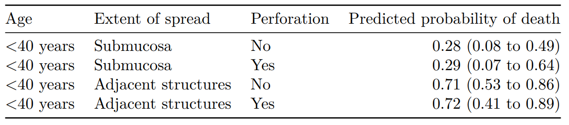
colon_s %>%
  glmmulti(dependent, explanatory) %>%
  boot_predict(newdata,
    estimate_name = "Predicted probability of death",
    R=100, boot_compare = FALSE,
    digits = c(2,3))

        Age    Extent of spread Perforation Predicted probability of death
1 <40 years           Submucosa          No            0.28 (0.00 to 0.52)
2 <40 years           Submucosa         Yes            0.29 (0.00 to 0.61)
3 <40 years Adjacent structures          No            0.71 (0.50 to 0.86)
4 <40 years Adjacent structures         Yes            0.72 (0.45 to 0.89)
Note that the number of simulations (R) here is low for demonstration purposes. You should expect to use 1000 to 10000 to ensure you have stable estimates.
Output to Word, PDF, and html via RMarkdown
Simulations are produced using bootstrapping and everything is tidily outputted in a table/dataframe, which can be passed to knitr::kable.
# Within an .Rmd file
```{r}
knitr::kable(table, row.names = FALSE, align = c("l", "l", "l", "r"))
```
Make comparisons
Better still, by including boot_compare==TRUE, comparisons are made between the first row of newdata and each subsequent row. These can be first differences (e.g. absolute risk differences) or ratios (e.g. relative risk ratios). The comparisons are done on the individual bootstrap predictions and the distribution summarised as a mean with percentile confidence intervals (95% CI as default, e.g. 2.5 and 97.5 percentiles). A p-value is generated on the proportion of values on the other side of the null from the mean, e.g. for a ratio greater than 1.0, p is the number of bootstrapped predictions under 1.0. Multiplied by two so it is two-sided. (Sorry about including a p-value).
Scroll right here:
colon_s %>%
  glmmulti(dependent, explanatory) %>%
  boot_predict(newdata,
    estimate_name = "Predicted probability of death",
    compare_name = "Absolute risk difference",
    R=100, digits = c(2,3))

        Age    Extent of spread Perforation Predicted probability of death      Absolute risk difference
1 <40 years           Submucosa          No            0.28 (0.00 to 0.52)                             -
2 <40 years           Submucosa         Yes            0.29 (0.00 to 0.62) 0.01 (-0.15 to 0.20, p=0.920)
3 <40 years Adjacent structures          No            0.71 (0.56 to 0.89)  0.43 (0.19 to 0.68, p<0.001)
4 <40 years Adjacent structures         Yes            0.72 (0.45 to 0.91)  0.43 (0.11 to 0.73, p<0.001)
What is not included?
It doesn’t yet include our other common models, such as coxph which I may add in. It doesn’t do lmer or glmer either. bootMer works well mixed-effects models which take a bit more care and thought, e.g. how are random effects to be handled in the simulations. So I don’t have immediate plans to add that in, better to do directly.
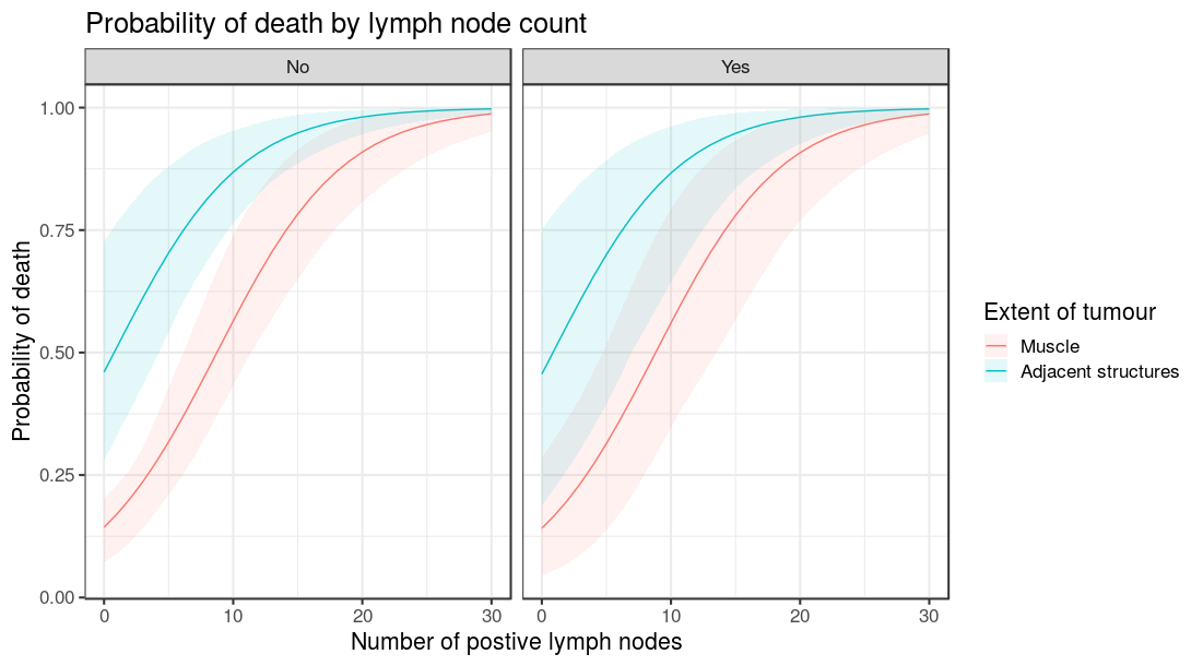
Plotting
Finally, as with all finalfit functions, results can be produced as individual variables using condense == FALSE. This is particularly useful for plotting
Your favourite package for getting model outputs directly into publication ready tables is now available on CRAN. They make you work for it! Thank you to all that helped. The development version will continue to be available from github.